Dispersion modelling: waste
- The text on this page is taken from an equivalent page of the IEHIAS-project.
As part of the EU-funded INTARESE project, which contributed to the development of this Toolbox, a case study was carried out to assess the health impacts of different waste management strategies in three study areas, in Italy, Slovenia and the UK.
In order to estimate exposures to airborne pollutants under the different management scenarios, dispersion modelling was carried out. Modelling was done for two pollutants (PM10 and NOx) arising from incinerators, landfills and waste transport.
Concentrations were modelled using the Atmospheric Dispersion Model System (ADMS-Urban), produced by [www.cerc.co.uk CERC]. This is a semi-Gaussian Lagrangian model. A key feature (compared to earlier models) is the incorporation of an up-to-date understanding of the atmospheric boundary layer, described in terms of the boundary layer depth and the Monin-Obukhov length, rather than by the Pasquill stability categories. Meteorological data requirements include temperature (°C), wind speed (m/s), wind direction (°), precipitation (mm), cloud cover (oktas), relative humidity (%), boundary layer height (m), and surface sensible heat flux (W/m2). Data are also required on the location and characteristics of the emission sources and receptors.
Incinerators and landfills

Incinerators and landfill sites were modelled as point sources (flares). Technical parameters required for this purpose included stack height (m), stack diameter (m), exit velocity (m/s), emission rate (m3/s), exit temperature (°C) and location of the stack.
For incinerators and landfill sites located in hilly terrain, the ADMS-Urban hill module was applied: this takes account of changes to dispersion patterns caused by the surrounding terrain. Postcode locations up to 10km away from the incinerators and landfill sites were specified as receptors.
Figure 1 shows typical annual mean NOx concentrations around an incinerator using hourly meteorological data.
Waste transport
Exposures from waste transport were modelled according to the following methodology:
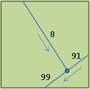
Details of the first two steps, route modelling and truck flows, are described elsewhere. They result in a detailed grid of traffic flows (and associated waste transported) across the study areas. The figure below illustrates a single grid cell, in which trucks serving 8 households on one road link converge with those serving 91 on another to give a total of waste from 99 households passing through the cell.


Step 3 Estimating emissions
In step 3, emissions from the truck flows in each grid are estimated. This is done by computing:
E = Σa [(2*Ha * Wh / Vt) * La * Ft]
where:
E = total annual emissions (grammes) from the gridcell
Ha is the number of households served by trucks passing along road segment a
Wh is the average amount of waste produced per household (tonnes/year)
Vt is the average capacity (tonnes) of a single truck
La is the length of road segment a (metres);
Ft is the emission factor (grammes/km) for an average truck
Note that the length is doubled to take account of the need for each truck to carry out a return trip.
The table below shows results for the example grid cell:
| Number of households served (Ha) | Average waste produced (Wh) | Waste transported (a * b) | Average truck capacity (Vt) | Number of truck trips (c/d) | NO2 emission factor (Ft) | Unit NO2 emissions (e*f) | Road segment length (La) | Total NO2 emissions (g*h/1000) |
|---|---|---|---|---|---|---|---|---|
| a | b | c | d | e | f | g | h | i |
| 8 | 1.45 | 11.6 | 8.0 | 2.9 | 5.636 | 16.4 | 80 | 1.31 |
| 91 | 1.45 | 132.3 | 8.0 | 33.1 | 5.636 | 186.4 | 10 | 1.86 |
| 99 | 1.45 | 143.9 | 8.0 | 36.0 | 5.636 | 202.8 | 10 | 2.03 |
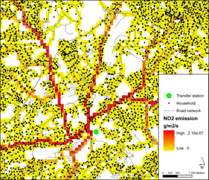
An example of a modelled emission grid is shown in Figure 2.
Step 4: Estimating concentrations
In step 4, concentrations are modelled at the receptor locations. Modelling was done by applying a GIS-based moving-window approach, using the ArcGIS command Focalsum to convert the emissions into concentrations (see a detailed description in Vienneau et al, 2009). Focalsum uses a kernel file to represent the pattern of weights in the window around each target cell. Concentrations in the target cell (Cj) are calculated as:
Cj = Σ (Eg * Kg)
where:
Eg is the modelled emissions from cell g
Kg is the weight applied to cell g in the kernel file
g represents all cells in the kernel file, centred on target cell j
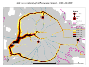
Kernel files were created by modelling a 100 x 100m grid cell with a reference emission rate of 1 g/m2/s in ADMS-Urban. Figure 3 shows the kernel file, as a graph, with the cell with the highest concentration being the centre cell with the 1 g/m2/s emission rate. Focalsum moves this window across the emission grid, converting the cells in concentrations (see Figure 4). Figure 5 shows results of the analysis in the Lazio area, Italy, as part of the waste case study.
References
- Vienneau, D., de Hoogh, K. and Briggs, D.J. 2009 A GIS-based method for modelling info air pollution exposures across Europe. Science of the Total Environment408, 255-266.
