Rapid modelling

The text on this page is taken from an equivalent page of the IEHIAS-project.

The purpose of rapid modelling is to provide quick and approximate estimates of health impacts, without the need to collect large volumes of data, to develop and text complex models, or to undertake lengthy and complex analyses.

The approach relies on the possibility of:

• using proxies for the phenomena of interest; or
• using analogues – i.e. ready-made and representative models from other applications; or
• building new, yet simple models that can estimate the small number of major factors that broadly determine the impacts.

Further information on, and examples of, these different approaches are given via the links in the panel to the left. A range of models and methods that can be used as a basis for rapid modelling are also provided in the Toolkit section of this Toolbox.

Proxies

Lack of measured data on the key phenomena of interest often means that proxies have to be used in studies of environment and health. Proxies such as distance from source or source intensity (e.g. distance to roads, road traffic volume) are widely employed in epidemiological studies to serve as exposure measures, where direct observations are unavailable. Likewise, measures of socio-economic status or education are used to represent the complex (but unmeasured) set of behavioural and contextual factors that help to determine susceptibility to environmental risk factors.

Proxies are similarly useful in carrying out screening studies for integrated impact assessment: their ready availability and ease of acquisition means that approximations may be made quickly and cheaply. They are especially valuable to represent changes in exposure.

As examples, we might use:

• regional land use as a proxy for exposure to pesticides or other contaminants from agriculture;
• population density as a proxy for exposure to urban air pollutants;
• occupation category as a proxy for exposures to industrial pollutants.

In defining proxies, we need to be cautious. Simple statistical association with the phenomena they are intended to represent (the objective) is often not sufficient, for the proxies are often used to indicate how the system will change in response to changing conditions or interventions (i.e. under different scenarios). This may involve extrapolating beyond the limits of existing data: in that range, the statistical relationships previously observed may no longer be valid. Statistical association also does not imply causality.

To be considered reliable, therefore, the proxies should be functionally related to the phenomena of interest. Even then, care is needed in using proxies, for the relationships involved are not always what is assumed, and may vary from one metric to another (see the example of traffic-related air pollution).

Confirmation of the association between the proxy and its objective is vital. If the proxies for exposure are to be used to provide estimates of potential health impacts, it is also important that a relevant exposure-response function is available (or can be deduced).

An example of traffic-related air pollution

Studies of traffic-related air pollution provide a good example of the need for, and dangers in using, proxies. One of the challenges these studies inevitably face is how to estimate exposures in the study populations. A number of issues make this especially difficult, including:

• The complex mix of transport-related emissions, and uncertainties about which pollutant should be targetted and what the relevant exposure metric should be;
• The need to obtain exposures for large study populations;
• The cost and limited potential to undertake personal monitoring;
• The sparseness of routine air pollution monitoring networks (as well as the limited range of pollutants that they cover);
• The limited capability for air pollution modelling available to many studies;
• The need to allow for the local variability in exposures which is often seen in urban areas;
• Concerns about effects of both long- and short-term exposures (and how these might interact).

In the face of these difficulties, studies have often had to make pragmatic decisions about study design, with the consequence that a wide range of measures and proxies have been used to represent exposures to the pollutant(s) of direct concern. Proxies for long-term exposures, for example, include:

• Land use category (e.g. city centre, high density residential, suburban);
• Distance from the nearest main road;
• Traffic volume on the nearest road;
• Road density (or traffic volume) in the surrounding neighbourhood;
• Self-reported measures of exposure (e.g. to traffic noise);
• Monitored concentrations of a marker pollutant (e.g. NO₂, PM₁₀) at the nearest routine monitoring site;
• Modelled concentrations of a marker pollutant (e.g. NO₂), using various different methods.

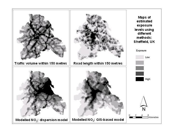
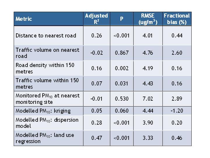
As a result of using these different exposure proxies, a wide variety of different exposure-response functions have been produced. In principle, these different metrics ought to tell a broadly similar story, so that the choice of exposure proxy should not be overly critical. In this case it would also be possible to convert the various measures into a common form, and thereby allow the exposure-response functions to be compared or combined. In practice, however, the different exposure proxies often seem to give very different results. The figure below, for example, illustrates how they can result in markedly different maps of air pollution. The table shows how their relationship with actual concentrations of (or exposures to) the real pollutants of interest (in this case, PM₁₀ concentration) can vary.

Proxies can certainly be useful, especially as a basis for a rough-and-ready approximation at the screening stage. They nevertheless need to be chosen with great care. Ideally, also, their relationship with the real exposure of interest ought to be clearly understood (and, if possible, quantified) before they are used.

Measures of correlation between different exposure proxies and measured annual average PM₁₀ concentration at 54 sites in London, UK

Analogues

For the purpose of screening, it may not be possible to obtain data that directly relate to the phenomena and populations of interest, nor to develop and apply models specifically designed for these situations. In these cases, however, it may be helpful (and possible) to use analogues – i.e. to ‘borrow’ data or models from other, comparable situations.

For example:

• if an exposure-response function is not available for the specific exposure (or health outcome or sub-population) of interest, one might be inferred from a similar one;
• if exposure distributions cannot be estimated in the specific micro-environment of interest, they might be inferred from an analogous one;
• if severity weights are not available for the specific disease (or population sub-group) of interest, they might be inferred from one with similar characteristics.

Analogues therefore have parallels with proxies (see link to left), and share many of the same issues. They differ in that, while proxies are functional substitutes for the phenomena of interest, analogues are extrapolations from similar (but functionally unrelated) situations. We therefore have to choose analogues with great care, for their validity depends wholly on the extent to which they are comparable in behaviour. As with other methods of approximation, evidence to support their use is crucial; if this does not already exist, then some form of testing ought to be done to confirm that they are appropriate.

Developing simple models

Given the absence (or impracticability) of well-validated and sophisticated models, we may need to resort to simpler methods for the purpose of screening. In some cases simple alternatives may already exist; in other cases they may need to be developed. In either case, the guiding principle should be that the models provide a reliable and robust approximation of the processes and phenomena of interest.

In reality, developing simple models is not as difficult as might be expected. The behaviour of many environmental systems is dominated by a relatively small number of variables, so if these can be approximated then the overall responses of the system can be estimated with some degree of accuracy. Whatever the medium, for example, pollutant dispersion tends to be determined by just three factors: the distance (or time) between source and receptor, the persistence or stability of the pollutant, and the dilution or filtering capability of the medium or micro-environment. Reflecting this, pollutant concentrations typically show quite clear spatial patterns that reflect, first and foremost, the source distributions and, secondly, the direction and gradient of dispersal. As a consequence, general pollution patterns can often be predicted relatively reliably from information on source distribution or intensity and basic environmental characteristics (e.g. wind direction, water flow, slope angle). Likewise, exposure or intake of any pollutant depends primarily on the extent to which the pollutants can penetrate or accumulate within the micro-environments where people spend their time, and the amount of time people spend there. This, too, can usually be approximated from simple information on the character of the micro-environment (e.g. ventilation conditions) and general time-activity data.

A useful, encompassing framework for this type of rapid estimation is given by the concept of Intake Fractions. This expresses the causal chain between source and intake in the form of a simple equation, and because of its generality previous estimates of intake fractions can be used to approximate exposures under different scenarios. A range of tools is also available for modelling links within this chain (e.g. from source to concentration, or concentration to exposure). Links are provided under 'See also' below.

See also

• Focal sum modelling in IEHIAS
• Land use regression in IEHIAS
• INDEX: indoor exposure model
• EMF path loss models
• Intake fractions