Multimedia models in IEHIAS
- The text on this page is taken from an equivalent page of the IEHIAS-project.
Multimedia models calculate the distribution of a chemical among different environmental compartments. These models usually treat environmental media, such as air, surface water and sediments, as uniformly mixed, steady state sub-systems; transport processes are described by simple equations based on measured or, more commonly, estimated parameters to describe transport rates between the different compartments.
Scope
Purpose:
Multimedia fate models are used to simulate the transport and transformation of chemicals through a range of different environmental media (e.g. air, water, soil). They are often applied to toxic substances which may persist in the environment for long periods of time, and thus offer the possibility of human exposure (or environmental damage) through a number of different routes.
Boundaries:
These models calculate concentrations of chemicals or other pollutants in varioius environmental media (soil, plants, water, air) or other compartments (e.g. buildings, geographic regions). Models can be applied at a wide range of scales, from micro-environmental to global, and over a range of timescales.
Method description
Input:
Required inputs include relevant transfer factors (e.g. partition or bioconcentration factors), describing the rates of transfer between and/or accumulation in different environmental compartments. Data are also needed on the initial releases of the agent into the system, and losses out of the system (e.g. by export).
Output:
The output of a multimedia model generally is an exposure concentration.
Rationale:
Multimedia models are based on transfer factors, such as partitioning or bioconcentration factors, and environmental concentrations of contaminants. For example, the bioconcentration of organic pollutants in fish is often derived from empirical bioconcentration factors or via an estimation equation which itself is obtained using observed correlations between the bioconcentration factor and the octanol-water partition coefficient . The bioaccumulation factor, however, can also be modeled, taking into account factors such as the trophic level, growth dilution and biomagnification. The use of such estimation methods is convenient because it allows for the assessment of many chemicals for which detailed empirical data do not exist.
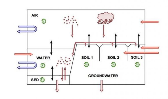
The general structure of a multimedia fate model is illustrated below (from Struijs and Peijnenburg 2002):
Method:
Multimedia environmental fate models may take various forms. Simpler models are typically in the form of a mass balance model, which assumes complete dispersion and mixing within each compartment and steady state conditions. Each compartment is described by a set of transfer functions which determine the rate or efficiency of transfer into and from neighbouring (or connected) compartments, and residence times within the compartment.
The general form of the model is thus:
where: Vi is the volume of the compartment i;
Ci is the concentration of the chemical in compartment i;
t is time;
Infi is inflow of the chemical into compartment i by emission from internal sources or import from outside the system;
Exfi is outflow of the chemical from compartment i by export outside the system;
Degi is loss by degradation (decomposition, decay) within compartment i;
Depi is loss by deposition (or other forms of immobilidation) within compartment i;
Excij is the exchange between compartments i and j.
Detailed formulation of the model inevitably depends on the characteristics of the chemical, the environmental media (compartments) concerned, and the processes that are relevant, as well as the spatial scale of analysis and time step used for modelling. Likewise, models become more complex where the assumptions of steady state and complete mixing are relaxed.
Examples of simple multi-compartment fate models are provided by multi-room indoor air models.
References
Hertwich, E.G., Jolliet, O., Pennington, D.W., Hauschild, M., Schulze, C., Krewitt, W. and Huijbregts, M.A.J. 2002 Fate and exposure assessment in the life cycle impact assessment of toxic chemicals. In: Life-cycle impact assessment: striving towards best practice (Udo de Haes, H.A., Finnveden, G., Goedkoop, M., Hauschild, M., Hertwich, E.G., Hofstetter, P., Jolliet, O., Klöpffer, W., Krewitt, W., Lindeijer, E., Müller-Wenk, R., Olsen, S.I., Pennington, D.W., Potting, J. and Steen, B., eds). Pensacola, Florida: Society of Environmental Toxicology and Chemistry (SETAC), pp 101-122.
Mackay, D. and Boethling,R.S. (eds) 2000 Handbook of property estimation methods for chemicals: environmental and health sciences. Boca Raton: CRC Press.
Struijs, J. and Peijnenburg, W.J.G.M. 2002 Predictions by the multimedia fate model Simplebox compared to field data. Intermedia concentration ratios of twp phthalate esters. RIVM Report 60722008. Bilthoven: RIVM.

