EU age/sex stratified population: 100 metre grid: Difference between revisions
No edit summary |
mNo edit summary |
||
| (3 intermediate revisions by one other user not shown) | |||
| Line 28: | Line 28: | ||
Data are based on ETRS89 Lambert Azimuthal Equal Area projection with parameters: latitude of origin 52° N, longitude of origin 10° E, false northing 3 210 000.0 m, false easting 4 321 000.0 m. | Data are based on ETRS89 Lambert Azimuthal Equal Area projection with parameters: latitude of origin 52° N, longitude of origin 10° E, false northing 3 210 000.0 m, false easting 4 321 000.0 m. | ||
* | If a country only has a single zip file (e.g. be.zip or dk_0.zip), you can simply unzip it and use. However, if a country is large, it has several zip files, which are zipped twice. First, you have to unzip all files of a country (e.g. at.zip.001.zip and at.zip.002.zip). This will produce several volumes of a larger zip file (e.g. at.zip which has volumes at.zip.001 and at.zip.002). Merge these volumes and then unzip the country file at.zip to produce the actual ascii files. | ||
* | |||
* | We recommend that you use 7zip program for unzipping! | ||
* | |||
* | * Austria {{#l:at.zip.001.zip}}{{#l:at.zip.002.zip}} | ||
* | * Belgium {{#l:be.zip}} | ||
* | * Czech Republic {{#l:cz_0.zip.001.zip}}{{#l:cz_0.zip.002.zip}} | ||
* | * Denmark {{#l:dk_0.zip}} | ||
* | * Estonia {{#l:ee_0.zip}} | ||
* | * Finland {{#l:fi_0.zip.001.zip}}{{#l:fi_0.zip.002.zip}}{{#l:fi_0.zip.003.zip}} | ||
* | * France {{#l:fr.zip.001.zip}}{{#l:fr.zip.002.zip}}{{#l:fr.zip.003.zip}}{{#l:fr.zip.004.zip}}{{#l:fr.zip.005.zip}}{{#l:fr.zip.006.zip}}{{#l:fr.zip.007.zip}}{{#l:fr.zip.008.zip}}{{#l:fr.zip.009.zip}}{{#l:fr.zip.010.zip}} | ||
* | * Germany {{#l:de.zip.001.zip}}{{#l:de.zip.002.zip}}{{#l:de.zip.003.zip}}{{#l:de.zip.004.zip}}{{#l:de.zip.005.zip}}{{#l:de.zip.006.zip}} | ||
* | * Great Britain {{#l:gb_0.zip.001.zip}}{{#l:gb_0.zip.002.zip}}{{#l:gb_0.zip.003.zip}} | ||
* | * Greece {{#l:gr_0.zip.001.zip}}{{#l:gr_0.zip.002.zip}} | ||
* | * Hungary {{#l:hu_0.zip.001.zip}}{{#l:hu_0.zip.002.zip}} | ||
* | * Ireland {{#l:ie_0.zip}} | ||
* | * Italy {{#l:it.zip.001.zip}}{{#l:it.zip.002.zip}}{{#l:it.zip.003.zip}}{{#l:it.zip.004.zip}}{{#l:it.zip.005.zip}} | ||
* | * Lithuania {{#l:lt_0.zip}} | ||
* | * Luxembourg {{#l:lu_0.zip}} | ||
* | * Malta {{#l:mt_0.zip}} | ||
* | * the Netherlands {{#l:nl_0.zip}} | ||
* | * Norway? Northern Ireland? {{#l:ni_0.zip}} | ||
* | * Poland {{#l:pl_0.zip.001.zip}}{{#l:pl_0.zip.002.zip}}{{#l:pl_0.zip.003.zip}}{{#l:pl_0.zip.004.zip}} | ||
* | * Portugal {{#l:pt_0.zip}} | ||
* Slovakia {{#l:sk.zip}} | |||
* Slovenia {{#l:si_0.zip}} | |||
* Spain {{#l:es_0.zip.001.zip}}{{#l:es_0.zip.002.zip}}{{#l:es_0.zip.003.zip}}{{#l:es_0.zip.004.zip}}{{#l:es_0.zip.005.zip}}{{#l:es_0.zip.006.zip}} | |||
* Sweden {{#l:se_0.zip.001.zip}}{{#l:se_0.zip.002.zip}}{{#l:se_0.zip.003.zip}} | |||
*[http://www.sciencedirect.com/science/article/pii/S0034425706005037 Dasymetric modelling of small-area population distribution using land cover and light emissions data. Remote Sensing of Environment.] Briggs D.J., Gulliver J., Fecht D. and Vienneau D.M. 2007. 108(4):451-466. | *[http://www.sciencedirect.com/science/article/pii/S0034425706005037 Dasymetric modelling of small-area population distribution using land cover and light emissions data. Remote Sensing of Environment.] Briggs D.J., Gulliver J., Fecht D. and Vienneau D.M. 2007. 108(4):451-466. | ||
*[http://link.springer.com/article/10.1007%2Fs11111-010-0108-y A population density grid of the European Union, Population and Environment]. Gallego F.J. 2010. 31: 460-473. | *[http://link.springer.com/article/10.1007%2Fs11111-010-0108-y A population density grid of the European Union, Population and Environment]. Gallego F.J. 2010. 31: 460-473. | ||
==See also== | |||
{{IEHIAS}} | |||
Latest revision as of 19:02, 25 September 2014
- The text on this page is taken from an equivalent page of the IEHIAS-project.


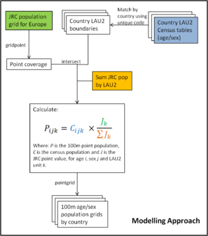
Even the highest resolution, LAU 2 level population data may be too coarse for some health risk assessments. Spatial modelling, therefore, may be required to disaggregate these totals to a finer grid. This has been done in several projects using land cover data as a basis for disaggregation (Briggs et al. 2007; Gallego 2010). Here the JRC population density grid (Gallego 2010) was enhanced by incorporating the age categories for both males and females from the census.
The modelling approach is illustrated below. Modelling involved proportioning the LAU2 level age/sex stratified data to the 100m cell on the basis of the JRC grid. Up to 28 grids (14 male and 14 female) were produced for each country depending on the structure of the age groups in the source tables.
Warning: These data are presented here at the 100m to offer flexibility in computing small area estimates at different spatial scales, however should not be taken to reflect population counts at the 100m level. Due to the lack of small area population data such as postcodes across Europe, these data were only validated for GB. Correlations (r) for total population were 0.92, 0.91 and 0.86 at the district, ward and 1km level, respectively. No correlation was found at the output area level. Similar modelling with validation found comparable results (Briggs et al. 2007), indicating that the 100m estimates could be reasonably aggregated to the 1km level.
Source / Reference
Three main sources of data were used to create these population grids:
- Small area census data
- Small area administrative boundaries (EuroBoundaryMap 1:1,000,000 January 2006 release)
- JRC population grid (version 4)
See also
Instructions:
Each country zip file contains up to 28 ascii files. To import into ArcGIS use the ASCII TO RASTER tool, or for ArcInfo use ASCIIGRID with the FLOAT option to create floating point grids.
Data are based on ETRS89 Lambert Azimuthal Equal Area projection with parameters: latitude of origin 52° N, longitude of origin 10° E, false northing 3 210 000.0 m, false easting 4 321 000.0 m.
If a country only has a single zip file (e.g. be.zip or dk_0.zip), you can simply unzip it and use. However, if a country is large, it has several zip files, which are zipped twice. First, you have to unzip all files of a country (e.g. at.zip.001.zip and at.zip.002.zip). This will produce several volumes of a larger zip file (e.g. at.zip which has volumes at.zip.001 and at.zip.002). Merge these volumes and then unzip the country file at.zip to produce the actual ascii files.
We recommend that you use 7zip program for unzipping!
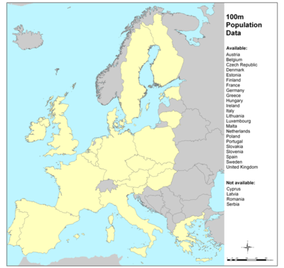
- Austria
 at.zip.001
 at.zip.002
 - Belgium
 be
be - Czech Republic
 cz_0.zip.001
 cz_0.zip.002
 - Denmark
 dk_0
dk_0 - Estonia
 ee_0
ee_0 - Finland
 fi_0.zip.001
 fi_0.zip.002
 fi_0.zip.003
 - France
 fr.zip.001
 fr.zip.002
 fr.zip.003
 fr.zip.004
 fr.zip.005
 fr.zip.006
 fr.zip.007
 fr.zip.008
 fr.zip.009
 fr.zip.010
 - Germany
 de.zip.001
 de.zip.002
 de.zip.003
 de.zip.004
 de.zip.005
 de.zip.006
 - Great Britain
 gb_0.zip.001
 gb_0.zip.002
 gb_0.zip.003
 - Greece
 gr_0.zip.001
 gr_0.zip.002
 - Hungary
 hu_0.zip.001
 hu_0.zip.002
 - Ireland
 ie_0
ie_0 - Italy
 it.zip.001
 it.zip.002
 it.zip.003
 it.zip.004
 it.zip.005
 - Lithuania
 lt_0
lt_0 - Luxembourg
 lu_0
lu_0 - Malta
 mt_0
mt_0 - the Netherlands
 nl_0
nl_0 - Norway? Northern Ireland?
 ni_0
ni_0 - Poland
 pl_0.zip.001
 pl_0.zip.002
 pl_0.zip.003
 pl_0.zip.004
 - Portugal
 pt_0
pt_0 - Slovakia
 sk
sk - Slovenia
 si_0
si_0 - Spain
 es_0.zip.001
 es_0.zip.002
 es_0.zip.003
 es_0.zip.004
 es_0.zip.005
 es_0.zip.006
 - Sweden
 se_0.zip.001
 se_0.zip.002
 se_0.zip.003
- Dasymetric modelling of small-area population distribution using land cover and light emissions data. Remote Sensing of Environment. Briggs D.J., Gulliver J., Fecht D. and Vienneau D.M. 2007. 108(4):451-466.
- A population density grid of the European Union, Population and Environment. Gallego F.J. 2010. 31: 460-473.