Bayes (Hierarcical Bayesian model)

This page describes utilization of Hierarcical Bayesin method. The following page briefly introduces theory behind the method, and illustrates the use the method by examples.

Introduction

The Bayesian method

The Bayes method is based on the bayesian rule. The following equations can be found from the reference 1, pages 7-8. The Bayesian rule is:

p(θ,y) = p(θ)p(y|θ)

,where p(θ) is prior distribution and on p(y|θ) is distribution acquired from the data. By contidionalizing θ with y (which is known), we get:

p(θ|y) = p(θ)p(y|θ) / p(y)

By conditionalizing this way, we obtain p(θ|y), which is prior probability conditionalised by the data. This is also called posterior probability. With these equations, we can adjust presuppositions about probability density function of the data using data itself. As a end result we obtain upgraded probability density function, which is called posterior density.   

Posterior distribution ~ prior distribution x distribution estimated by the data

Hierarcical Bayesian method

We create an example of the method in this article. We study dioxin concentrations in different sea area which we assume to be share a similar form of distribution. In other words, we assume that the concentraions in different areas are samples of the total concentration distribution. Thus, we can use observations of concentrations in all areas to estimate concentrations in one particular area of interest. This means conditionalizing observated values to certain parameters. We assume probabilites to these parameters with new parameters, which are called hyperparameters.

There is an extensive explanation of the idea and the method in reference 1, pages 117-121, and you can find a picture of the method in page 119. In our example, we try to create a model which gives us a relatively accurate concentration estimate for all different areas.

Material and methods

Methods

The method used herein is called hierarcical Bayes method. Theory can be read from reference 1. We used WinBUGS and R as a modelling tool. 

http://www.mrc-bsu.cam.ac.uk/bugs/

You can get the program and updates from the address above. They also include quite extensive manuals. You need to copy the text to WinBUGS to a new file, and select decode from tools menu and follow the manual. 

Table 1. Names of the variables and parameters in the model. 

Variable	Distribution	Nature	Parameters	Definition	Description
alpha.tau	gamma	stocastic	10^-3		Parameter of accuracy
alpha.c	norm	stocastic	(0,10^-6)		Mean
alpha0		calculated		(a.c)-(b.c)*xbar	Starting level
alpha[i]	norm	stocastic	(a.c,a.t)		Constant term
beta.tau	gamma	stocastic	10^-3		Parameter of accuraty for slope
beta.c	norm	stocastic	(0,10^-6)		Mean value of slope
beta[i]	norm	stocastic	(b.c,b.t)		Slope
mu[i,j]		calculated		a[i]+b[i]*(x[j]-xbar)	Estimation for concentration
x[j]		constant		input	Age categories
tau.c	gamma	stocastic	10^-3		Parameter of accuracy
sigma		calculated		1/sqrt(tau.c)	Dispersion term
y[i,j]	norm	stocastic	(mu[i,j],tau.c)		Estimate for concentration without  observation

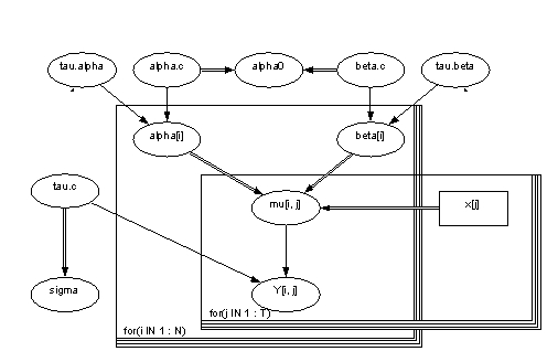
Picture 1. Picture of the model in Win BUGS

Material

The data we used in our example consists of dioxin concentration of herring with ages, sizes and location

We create a model similar to example model in WinBUGS. Variables are analogous as demonstrated below:
Variables:

Weight of rat = Concentration of herring
Age of rat = Age of herring
Number of rat (specimen #) = Location

We ran the model with Win BUGS with herring data, and examined the distribution of variables of interest.In rat example the model estimates distributions for weight for each rat. In our model we estimate concentration distributions for each location.

Results

Descriptive statistics

Kuva 2. Age against concentration in herring

Image:Ikä_vs_poitoisuus_silakka.jpg

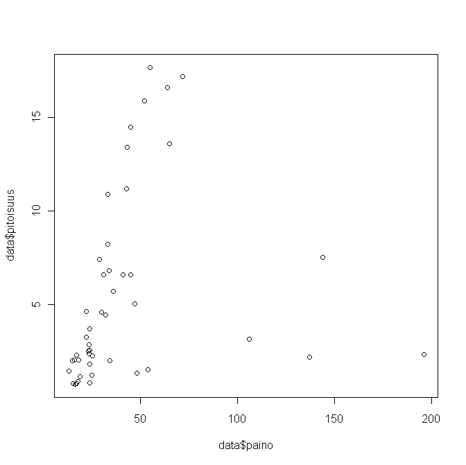
Kuva 3.Weight against concentration in herring

Results of a linear regression model, where concentraition is explained with age and weight

Call:
lm(formula = pitoisuus ~ ikä + paino, data = data)

Residuals:
Min 1Q Median 3Q Max
-7.9395 -1.3808 -0.1211 1.2573 6.4274

Coefficients:
Estimate Std. Error t value Pr(>|t|)
(Intercept) -1.68568 0.78077 -2.159 0.0363 *
ikä 1.66347 0.14978 11.106 2.39e-14 ***
paino -0.03660 0.01205 -3.038 0.0040 **
---
Signif. codes: 0 ‘***’ 0.001 ‘**’ 0.01 ‘*’ 0.05 ‘.’ 0.1 ‘ ’ 1

Residual standard error: 2.575 on 44 degrees of freedom
Multiple R-squared: 0.7495, Adjusted R-squared: 0.7381
F-statistic: 65.82 on 2 and 44 DF, p-value: 5.952e-14

Huomataan siis että ikä ja paino merkitseviä selittäjiä.

We notice that both age and weight are significant explanators.

Results of WinBUGS calculations

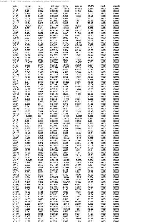
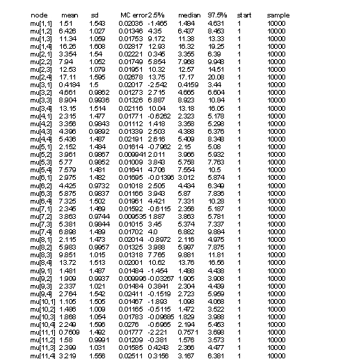
Tables 2 and 3 represent results of our model. In Y[1,2], the first parameter denotes to concentraion of on year old herring in location one (=1), and the second parameter denotes to age category (=2). Thus, the first parameter stands for location and the second parameter for age. Some values (confidence intervall 2.5%) are less than zero (which is not plausible as concentrations can not be negative), but we can control this by not allowing values below zero in our model. In table 3 there are ages divided into four categories (including three years each) and estimates for concentrations.  Median values do not have values below zero but 2.5% CI has negative values. Estimates in table 2 are for missing values only. Medians seem to be quite good estimates but the confidence intervalls span very wide due to lack of data.

Table 2. List of results for herringdata with one year age intervals (WinBUGS). 

Table 3. List of results for dioxin concentration in herring with three year age intervall (Win BUGS)

Syntaxes and iterations 

Attached are the code of the model (model1, noodle_1 and data_1). There are age groups 1-4 and data_1 for each age categories, as well as inits (if we don't want to simulate them).

All codes open with WinBUGS program and are updated freely. Simulations are using model1 and data_1 and they are working with inits. Similar model can be found in examples (help menu)  vol1 Rars. Setting a limit is done by adding syntax I(0,) to the end of distribution definition.

Running the model:

You need to open three windows. Under model find model specification, under inference find samples, and under model find update. With these, you can run the same calculations as we just did.

You can find the files from:

N:\Huippuyksikko\Tutkimus\R55_PMvsDioxin\MeHgvsOmega-3\mallit\Bayes\Aiemmat ajot ja pähkäilyt

Conculsions

We can compare the results with data and draw conclusions. The median estimates seem to have pretty ok values compared the the original data.

Rat example

This model can be found from WinBUGS help page. Our example is based directly to this model.

Rats: a normal hierarchical model

This example is taken from section 6 of Gelfand et al (1990), and concerns 30 young rats whose weights were measured weekly for five weeks. Part of the data is shown below, where Yij is the weight of the ith rat measured at age xj.

Weights Yij of rat i on day xj
xj = 8 15 22 29 36
__________________________________
Rat 1 151 199 246 283 320
Rat 2 145 199 249 293 354
.......
Rat 30 153 200 244 286 324

A plot of the 30 growth curves suggests some evidence of downward curvature.

The model is essentially a random effects linear growth curve

Yij ~ Normal(i + i(xj - xbar), c)

i ~ Normal(c, )

i ~ Normal(c, )

where xbar = 22, and  represents the precision (1/variance) of a normal distribution. We note the absence of a parameter representing correlation between i and i unlike in Gelfand et al 1990. However, see the Birats example in Volume 2 which does explicitly model the covariance between i and i. For now, we standardise the xj's around their mean to reduce dependence between i and i in their likelihood: in fact for the full balanced data, complete independence is achieved. (Note that, in general, prior independence does not force the posterior distributions to be independent).

c , , c , , c are given independent "noninformativepriors, with two alternatives considered for  and : prior 1 is uniform on the scale of the standard deviations  = 1/sqrt() and  = 1/sqrt(), and prior 2 is a gamma(0.001, 0.001) on the precisions  and . Interest particularly focuses on the intercept at zero time (birth), denoted 0 = c - c xbar.

Graphical model for rats example (using prior 1):

BUGS language for rats example:

Note the use of a very flat but conjugate prior for the population effects: a locally uniform prior could also have been used.

Data list(x = c(8.0, 15.0, 22.0, 29.0, 36.0), xbar = 22, N = 30, T = 5,
Y = structure(
.Data = c(151, 199, 246, 283, 320,
145, 199, 249, 293, 354,
147, 214, 263, 312, 328,
155, 200, 237, 272, 297,
135, 188, 230, 280, 323,
159, 210, 252, 298, 331,
141, 189, 231, 275, 305,
159, 201, 248, 297, 338,
177, 236, 285, 350, 376,
134, 182, 220, 260, 296,
160, 208, 261, 313, 352,
143, 188, 220, 273, 314,
154, 200, 244, 289, 325,
171, 221, 270, 326, 358,
163, 216, 242, 281, 312,
160, 207, 248, 288, 324,
142, 187, 234, 280, 316,
156, 203, 243, 283, 317,
157, 212, 259, 307, 336,
152, 203, 246, 286, 321,
154, 205, 253, 298, 334,
139, 190, 225, 267, 302,
146, 191, 229, 272, 302,
157, 211, 250, 285, 323,
132, 185, 237, 286, 331,
160, 207, 257, 303, 345,
169, 216, 261, 295, 333,
157, 205, 248, 289, 316,
137, 180, 219, 258, 291,
153, 200, 244, 286, 324),
.Dim = c(30,5)))

(Note: the response data (Y) for the rats example can also be found in the file ratsy.odc in rectangular format. The covariate data (X) can be found in S-Plus format in file ratsx.odc. To load data from each of these files, focus the window containing the open data file before clicking on "Data" from the "Model" menu.)

Inits1 list(alpha = c(250, 250, 250, 250, 250, 250, 250, 250, 250, 250, 250, 250, 250, 250, 250,
250, 250, 250, 250, 250, 250, 250, 250, 250, 250, 250, 250, 250, 250, 250),
beta = c(6, 6, 6, 6, 6, 6, 6, 6, 6, 6, 6, 6, 6, 6, 6,
6, 6, 6, 6, 6, 6, 6, 6, 6, 6, 6, 6, 6, 6, 6),

alpha.c = 150, beta.c = 10,
tau.c = 1, sigma.alpha = 1, sigma.beta = 1)

Inits2 list(alpha = c(250, 250, 250, 250, 250, 250, 250, 250, 250, 250, 250, 250, 250, 250, 250,
250, 250, 250, 250, 250, 250, 250, 250, 250, 250, 250, 250, 250, 250, 250),
beta = c(6, 6, 6, 6, 6, 6, 6, 6, 6, 6, 6, 6, 6, 6, 6,
6, 6, 6, 6, 6, 6, 6, 6, 6, 6, 6, 6, 6, 6, 6),
alpha.c = 150, beta.c = 10,
tau.c = 1, tau.alpha = 1, tau.beta = 1)

Results

A 1000 update burn in followed by a further 10000 updates gave the parameter estimates:

node mean sd MC error 2.5% median 97.5% start sample
alpha0 106.6 3.65 0.04151 99.43 106.5 113.9 1001 10000
beta.c 6.185 0.1102 0.001294 5.967 6.185 6.404 1001 10000
sigma 6.074 0.4673 0.007724 5.247 6.044 7.068 1001 10000

Using Prior 2 (not recommended) has negligible impact

These results may be compared with Figure 5 of Gelfand et al 1990 --- we note that the mean gradient of independent fitted straight lines is 6.19.

Gelfand et al 1990 also consider the problem of missing data, and delete the last observation of cases 6-10, the last two from 11-20, the last 3 from 21-25 and the last 4 from 26-30. The appropriate data file is obtained by simply replacing data values by NA (see below). The model specification is unchanged, since the distinction between observed and unobserved quantities is made in the data file and not the model specification.

click on one of the arrows to open the data for the missing value analysis

Gelfand et al 1990 focus on the parameter estimates and the predictions for the final 4 observations on rat 26. These predictions are obtained automatically in BUGS by monitoring the relevant Y[] nodes. The following estimates were obtained:

We note that our estimate 6.58 of bc is substantially greater than that shown in Figure 6 of Gelfand et al 1990. However, plotting the growth curves indicates some curvature with steeper gradients at the beginning: the mean of the estimated gradients of the reduced data is 6.66, compared to 6.19 for the full data. Hence we are inclined to believe our analysis. The observed weights for rat 26 were 207, 257, 303 and 345, compared to our predictions of 204, 250, 295 and 341.

Table 4. Original data for herring

Age	Weight	Concentration
2	15	1.96
4	23	2.49
6	31	6.58
7	43	13.4
11	71.7	17.2
2	17,6	0.876
3	25.2	2.22
3	34.1	1.99
5	54	1.5
6	137	2.18
2	18	2
2	24	2.52
6	33	8.23
9	52	15.9
11	64	16.6
2	16.3	0.704
4	23.6	2.84
7	34	6.79
9	45	14.5
12	65	13.6
2	17	2.29
3	24	3.67
7	33	10.9
8	42.9	11.2
9	55	17.7
1	15.3	0.733
3	23.5	2.35
5	30	4.59
7	41	6.59
3	15.8	2.02
6	22	4.6
7	29	7.4
7	47	5.03
6	144	7.52
1	19	1.13
3	25	1.186
5	36	5.7
2	13	1.42
5	22	3.25
6	32	4.44
8	34	6.58
10	106	3.13
1	17	0.768
3	24	1.79
2	24	0.782
3	48	1.29
7	196	2.31