Spatial population modelling example
- The text on this page is taken from an equivalent page of the IEHIAS-project.
Reliable information on the location and distribution of the population is essential in many health impact studies and, in particular, for exposure and risk assessment where it is needed to facilitate the calculation of population-level exposures. Census data provide regularly updated information on population counts and demographics in the EU and elsewhere around the world. The way in which census tracts are defined, however, can limit the value of these data for assessing exposure.
Dasymetric disaggregation is an established approach for generating small-area population estimates. Dasymetric disaggregation, or dasymetric mapping, is an intelligent disaggregation procedure that incorporates ancillary data to facilitate the areal interpolation process. It differs from choropleth mapping in that areas are defined based on the actual spatial distribution of the variable being mapped, rather than administrative or other arbitrary units. This technique has gained popularity with the increasing availability of satellite imagery and improved methods of utilising Earth Observation (EO) data in a GIS.
For population modelling, land cover data are particularly useful as a means by which residential areas can be distinguished from non-residential areas. In polycategorical dasymetric disaggregation, specific disaggregation weights can be derived for individual land cover types to reflect population density. The challenge in this approach is to devise an appropriate set of weights that can be applied to the land parcels (or other ancillary data) to reflect real population densities. We would expect, for example, more people to live in high and low density residential areas compared to rural ones; thus the weights should be ordered high density residential > low density residential > rural. Weights may be defined using selective sampling or, as in this example, using regression analysis.
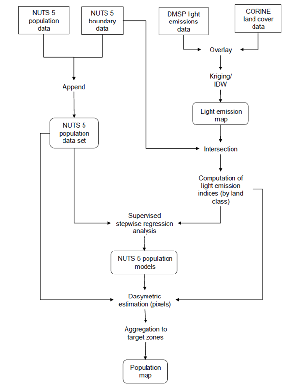
In an EU-wide application, Briggs et al (2007) developed a model that incorporates ancillary data, specifically EO night-time light intensity data and CORINE land cover, in a GIS-based regression approach to disaggregate NUTS 5 (~LAU-2) census totals to a resolution of 1km2. As illustrated in the flow diagram below, European light emission data from the DMSP satellites were resampled and modelled using kriging and inverse distance weighting to provide a 200-m resolution light emissions map. This was matched to CORINE land cover classes and regression analysis used to derive models of relationships between census population counts and land cover area and light emissions. Both national and EU scale models were developed, with R2 for predicted versus actual ppulation numbers typically in the order of 0.8-0.9. The resulting population models and map can be viewed here.
References
- Briggs D. J., Fecht D., Gulliver J., and Vienneau D. 2007 Dasymetric modelling of small-area population distribution using land cover and light emissions data. Remote Sensing of Environment 108:451-466.
