Piloting: Finding and evaluating data
- The text on this page is taken from an equivalent page of the IEHIAS-project.
Contents
Finding and evaluating data
Good data are clearly essential for any assessment. Rarely, however, are data initially collected or produced for the purpose of assessment - nor can many assessments wait until new, primary data are generated by purpose-designed studies or surveys. Instead, in most cases, assessments have to make use of data that already exist, and to supplement or enhance these as necessary through the use of modelling or estimation techniques.
Conducting a data review
Assessments are consequently servants of the available data, and have to be designed to make the best possible use of what exists. A vital purpose of feasibility testing is thus to review and evaluate the available data. This is not a question of simply applying some predefined criteria and deciding whether or not the data meet these requirements. The intention must be to identify what data do exist, and determine what can be done with them, and what resources might be needed to make this possible.
To ensure that the review is thorough, but does not lead us too far away from our initial purpose, it is therefore crucial to start by defining the key data we need and the criteria that they must satisfy (e.g. in terms of geographic coverage and resolution, timeframe, cost). Data sources should be evaluated against this list, and any deficiencies noted. In addition, however, possibilities offered by these data should also be identified, and if these imply other data needs (e.g. for the purpose of validation or to help make good their deficiencies), then these need to be added into the list and followed up. In this way a detailed log of the review can be maintained, which can be fed into the process of devising and discussing the assessment protocol. Examples, from case studies carried out during the development of this Toolbox, are given via the links below.
The links in the panel to the left provide access to useful sources, including inventories and metadatabases summarising relevant data in the EU.
Environmental and exposure data
Information on the exposures of the population to the environmental hazards of concern are essential in any environmental health impact assessment. Ideally, these would come from direct measurement or monitoring of the population, either using biomarkers or by personal monitoring. Unfortunately, this is rarely feasible, both because of the lack (and cost) of such monitoring, and because most assessments are concerned with situations that have not yet happened, or with past conditions which can no longer be directly observed. In the absence of such data, recourse is therefore often made to environmental monitoring data. Nevertheless, albeit to a lesser degree, these suffer from many of the same limitations: namely the sparseness of the data and their restriction only to existing and some past conditions. As a consequence most assessments ultimately rely on some form of modelling to estimate exposures under the various scenarios of interest.
None of this is to mean that direct measurements of exposure, dose or environmental conditions (e.g. concentrations) are not valuable for integrated environmental health impact assessments. In most cases, indeed, they are vital - either as inputs to models, or to validate models based on other predictors. Such data, however, are rarely sufficient. Most assessments also have to call on a range of other forms of environmental data, in order to estimate exposures and to model the way in which changes propagate through the causal chain. Thus, data are typically required on a wide range of environmental factors, such as the topography, weather, soil, hydrology and land cover.
Traditionally, most environmental data were obtained by ground-based field surveys. With the development of methods of remote sensing, however, airborne and satellite observations have become far more important, and these now provide the primary source for many types of environmental data. As survey and monitoring technologies have advanced, so the range, size and complexity of environmental databases has grown. Today, therefore, the main challenge is to find relevant data from the myriad of sources available, and to extract and combine them in an efficient way.
In Europe, the European Environment Agency provides an invaluable source of many data. At national level, environmental ministries and their associated agencies also hold, or can give access to, a wide range of data. Another valuable source, specific to environmental health, is the ExpoPlatform. Factsheets for many of these data (along with selected data sets) are provided in the Environmental data section of the Toolkit, and these give links to many of the data sources.
Representivity of environmental monitoring networks
Routine monitoring networks provide a valuable source of data on environmental conditions, which can be used in integrated assessments. Their ability truly to represent the full range of environmental conditions (or human exposures to them) is nevertheless limited, for the environment itself is highly variable, over both space and time, while monitoring is costly and technically constrained, so networks are limited both in their extent and what they measure. These limitations need to be borne in mind whenever monitoring data are used for integrated assessments - whether as a basis for exposure assessment in their own right, as inputs to models, or as a basis for model validation. By the same token, considerable care is needed in designing monitoring systems or measurement campaigns for the purpose of assessment.
Estimating representivity
Determining the representivity of monitoring networks is not easy. On the one hand, the concept of representivity is somewhat vague (and there is no agreement even about what to call it!), so that relevant measures are not always obvious (see references below). Simple statistical measures are available to estimate sample sizes. All such analyses, however, depend on assumptions about the underlying statistical distributions of the properties being measured - and these can only be deduced from the data provided by the existing monitoring network. Inadequacies in the sample design of this network inevitably means that these assumptions are uncertain. Unless additional monitoring can be carried out, at a sampling density sufficient to detect any unseen regularities or local variabilities in the environment, therefore, the estimates of sample requirements are likely to be unreliable (and in many cases to under-estimate the true sampling density that is required, or to define the most effective sampling configuration.
Nor, in the case of assessment, is the the need usually just to minimise the standard errors of the estimates. Instead, monitoring may have to ensure that:
hotspots and vulnerable population sub-groups are correctly identified; uncertainties are reasonably equal across different parts of the study area and population; a strong correlation exists between predicted and actual conditions across the whole study area/population; monitoring costs are kept within necessary limits. This implies the use of a number of different measures, reflecting different design criteria, to estimate representivity. Optimising them all is rarely possible, for the different criteria are to some extent in conflict, so trades off have to be made between them. Representivity is not an absolute, therefore, but depends on the needs of the study, and can only be judged in terms of context.
An illustration of many of these considerations, and an example of how different network designs can affect estimates of population exposures to environmental pollution is given in the attached document, on the representivity of air pollution monitoring networks. This was developed through a simulation exercise, using the SIENA urban simulator. A detailed report can be downloaded below.
Tools for sampling design
A number of tools to help design monitoring systems and sampling strategies exist, including the Visual Sample Plan (VSP), developed by Battelle Pacific Northwest National Laboratory. This provides an interactive and highly flexible, map-based system for estimating sample size and selecting between different sampling configurations, for a wide range of different user-defined purposes, including estimation of the sample mean, trend detection and exceedance analysis.
Exposure-response functions
Exposure response functions (ERF) describe quantitatively how much a certain health effect increases when the exposure of a certain stressor increases. The ERF needs to relate specifically to the exposure metric and health endpoint used in the assessment.
The ERF can be derived in a number of ways. Where a published and up-to-date ERF is available from an authoritative organisation, such as the World Health Organization, this should preferably be used. If not, a systematic review (including if appropriate a meta-analysis) should ideally be conducted to derive an ERF for the key impact pathways. Where this, too, is not possible, an alternative is to make use of the formal methods of an expert panel. Systematic reviews and expert panels are both time-consuming to design and run, so modified, less-time consuming versions may be more appropriate. Options include:
adopting the ERF used in previous HIAs; taking results from an already published and good-quality meta-analysis; using results from a key multi-centre study. If these informal methods are used it is advisable to consult expert(s) in the relevant policy field (not a formal expert panel).
These methods can be applied to animal and human studies. However, if applied to animal studies, extrapolation to humans is necessary. In this case, a qualitative assessment should first be carried out to evaluate whether an observed effect in animal studies applies to humans.
A protocol, giving guidelines on how to develop ERFs, is available via the link under See also, below. Figure 1 (below) provides a summery of this protocol and presents a checklist of questions that should be considered in order to derive an ERF.
An ERF data set, providing suggested exposure-response functions for common exposures and health endpoints is also included in the Data section of the Toolkit.

Figure 1. A checklist for deriving an ERF
Human biomonitoring data
Human biomonitoring (HBM) can be defined as "a method for assessing human exposure to chemicals (or their associated effects) by measuring these chemicals, their metabolites, or reaction products in human tissues or specimens such as blood, urine or hair'.
Role of HBM in integrated assessment
In many cases, HBM data has proved to be a valuable supplement to, or have even surpassed, estimates of exposure based on environmental measures. HBM directly measures the amount of a chemical substance in a person’s body, taking into account often poorly understood processes such as bioaccumulation, excretion, metabolism and the aggregate uptake variability through different exposure pathways. The data can therefore make a number of important contributions to integrated assessments:
They can provide more direct estimates of exposures to environmental contaminants than extrapolations from chemical concentrations in soil, air or water; They can help to quantify and understand the (otherwise hidden) links between exposure, internal dose and health reponse (see Figure 1); In this way, they can provide information on variations in, and help to identify determinants of, susceptibility in human populations.

Figure 1. The role of human biomonitoring in understansing exposure-dose-response relationships
Over the last decade or so, a wide variety of human biomarkers have been developed and tested. These provide the capability to assess exposures to, and health effects from, a range of different chemicals. Details of 15 biomarkers, representing some of the most common (classes of) chemicals are provided in the Toolkit section of this Toolbox (see links via Table 2, below). Further details are also available from the report, Biomarker review and development strategy, which can be downloaded below.
Table 2. Links to information for biomarkers of key chemicals
Biomarkers such as these have a number of specific characteristics that give them advantages over other sources of data:
- Biomarkers represent aggregate exposure and, if chosen wisely, can help to interpret and anlayse environmental health impacts of exposure mixtures;
- Biomarkers describe a continuum between exposure and health effects, and thus provide linked and consistent information on exposure-health relationships (Smolders et al. 2010b);
- New developments in related sciences, generally referred to as the “-omics” technologies, are creating novel opportunities for the discovery of new relationships between exposure and health effects;
- Biomarker data and PBPK models support one another, either by providing mechanistic understanding of the dose-metric, or by model validation of PBPK models (see PBPK modeling).
Sources of HBM data
With the growing recognition of the value of HBM data, a number of large population surveys have been initiated in recent years, both in Europe and more widely (Table 1). These can give a good idea of the typical levels of chemicals that are observed in the general population. In addition, many smaller, ad hoc studies have been undertaken, often focused on specific chemicals and population groups. As the example of surveys relating to blood-lead in the EU (see link below) indicates, however, combining data from these can face difficulties, because of differences in survey design and analytical methodology. Further information is also given in the Biomarkers inventory, which can be downloaded below.
| Country | Survey | URL |
|---|---|---|
| Belgium | Flemish CEH | http://www.milieu-en-gezondheid.be/English/index.html |
| Canada | CHMS | http://www.hc-sc.gc.ca/ewh-semt/contaminants/human-humaine/index-eng.php |
| Czech Republic | Environmental Health Monitoring | http://www.szu.cz/topics/environmental-health/environmental-health-monitoring |
| Germany | GerES | http://www.umweltbundesamt.de/gesundheit-e/survey/index.htm |
| International | COPHES project | http://www.eu-hbm.info/ |
| International | ESBIO inventory | http://www.hbm-inventory.org/scid/e-formv2/default.asp |
| International | WHO human milk monitoring | http://www.who.int/foodsafety/chem/pops/en/index.html |
| USA | NHANES | http://www.cdc.gov/exposurereport/ |
Table 1. A brief overview of some large scale HBM population surveys.
Case studies in human biomonitoring
Tags: Administrators -> 491 As part of the EU-funded INTARESE project, which contributed to the development of this Toolbox, a series of case studies were undertaken, aimed at exploring and illustrating the use of human biomonitoring data in integrated environmental health impact assessment. Summaries of the findings are given below, and links to more information are provided.
Data availability
Setting up an HBM study is logistically, financially and scientifically challenging. Integrated impact assessments, however, need to provide results relatively swiftly, and are usually severely constrained in terms of resources. They therefore need to make use of readily available data. The case-study on blood-lead concentrations showed that it is feasible to collect and use data from previous studies, and illustrates how this can be done. (Follow link to a description of the study here).
Describing the dose-effect continuum
One of the major advantages of human biomonitoring data is that they can provide consistent information spanning the links between exposure, intake, dose and health effect. A case-study on PAH exposure, simultaneously performed in Flanders and the Czech Republic, showed how combination of methods, ranging from emission modeling, through the use of biomarkers of exposure, to application of effect-markers can enhance understanding of the health impacts of road traffic (follow link to Exploring the full-chain approach for PAHs using 2 case studies in Flanders and the Czech Republic ![]() Exploring the full-chain approach for PAHs).
Exploring the full-chain approach for PAHs).
Identifying appropriate health outcomes
In a health impact assessment, the choice of the health endpoints has a crucial effect on the outcome of the assessment. A case-study on PCBs showed how benchmark dose modelling may be useful to identify the most sensitive endpoints (follow link to The Benchmark dose (BMD) approach for health effects of PCB exposure).
Interpreting human biomonitoring data
Tags: Administrators -> 501 Human biomonitoring data can rarely be interpreted in isolation. Apart from well-described examples, such as lead (Pb) in gasoline or methylmercury (MeHg) in seafood, biomarkers cannot usually be linked directly to a single source or exposure pathway, so do not necessarily reveal how exposures have occurred. Equally, while biomonitoring can provide invaluable information on current exposures and health effects, monitoring on its own does not provide a robust prediction of how exposures and effects may change under a potential future policy (or other) scenario. For these and other reasons, biomonitoring invariably needs to be linked to other forms of monitoring and modelling when used in health impact assessments.
One of the most important opportunities for such an approach is in the analysis of the links between exposure, dose and health effect. In recent years, physiologically based pharmacokinetic (PBPK) modelling has shown to be well-suited to calculate tissue doses of chemicals and their metabolites over a wide range of exposure conditions. Because these PBPK models are based on the human physiology and anatomy and summarise the behaviour of chemicals in the body, they are often considered to be more realistic than empirical models. PBPK modeling nevertheless faces a challenge in detecting and quantifying variation in source-to-dose relationships against the noise contributed by the wide range of other factors (e.g. variable exposures, activities, physiology, and pharmacokinetics) that operate within large (and often poorly characterised) human populations. Linking HBM data with PBPK models can therefore help to address the limitations of both technologies.
Linking PBPK modelling and HBM has led to a number of new conceptsd and tools for deriving health-based guidance values to support risk assessment and management. Amongst these, three are of particular note: biomonitoring equivalents, reverse dosimetry and repeated measurements.
More information can be found in the attached document 'Interpretation of HBM data', which can be downloaded below.
Biomonitoring equivalents
Biomonitoring Equivalents (BEs) are defined as the concentration of a chemical (or metabolite) in a biological medium consistent with defined exposure guidance values or toxicity criteria (including reference doses and reference concentrations, minimal risk levels or tolerable daily intakes). These exposure guidance values are estimates of the daily exposure to a chemical that are believed to be without appreciable health risks, and can be used by regulatory agencies as guidelines for making risk management decisions. BEs thus use available pharmacokinetic data and forward dosimetry to calculate levels of biomarkers associated with these exposure guidance values (Figure 1).
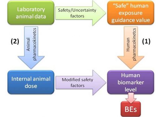

Figure 1. Determination of biomonitoring equivalents
Ideally, calculation of BEs is done using human pharmacokinetic data to relate external dose to biomarker concentrations (pathway 1 in Figure 1). However, when only animal-based pharmacokinetic information is available (pathway 2), this may be applied, taking into account the appropriate uncertainty or safety factors.
It needs to be stressed that BE values are screening values. Comparison of measured biomonitoring levels to BE values can provide an initial, indicative evaluation of the need for follow up for risk assessment, and whether there is a need for additional studies on exposure pathways, potential health effects, other aspects affecting exposure or risk, or other risk management activities.
The limitations of BE values need to be reognised. They are not diagnostic criteria or 'bright lines' between safe and unsafe levels, so do not directly identify at-risk groups. Nor can they be used to evaluate the likelihood of an adverse health effect in an individual or a population, so they are not a direct means of health impact assessment. Exposure guidance values are set at levels that are designed to be health-protective for daily exposure for a full lifetime of exposure, while, depending on the chemical, biomonitoring data may be informative only about recent exposure levels. An exceedance of the BE value in a single sample of blood or urine may or may not reflect continuing elevated exposure and does not imply that adverse health effects are likely to occur, but can serve as an indicator of relative priority for further risk assessment follow-up.
Reverse dosimetry
Reverse dosimetry provides a means of source identification for the interpretation of biomarker values. Establishing the relationship between biomarker data and environmental sources involves the reconstruction of past external exposure. Ths has been termed 'exposure reconstruction' or 'reverse dosimetry'. For this purpose, the PBPK model is reversed, and human biomonitoring data are back-transformed into equivalent exposure concentrations, by using pharmacokinetic data in combination with information regarding the nature of the potential exposures to infer the exposures that are likely to have led to the measured biomonitoring results.
The fundamental problem underlying reverse dosimetry is to relate a measured internal dose, or tissue concentration to an unmeasured external exposure or dose, and beyond that a range of putative sources. A major challenge in this approach is the need to take into account the inherent variability of the population from which the HBM data arises. As a consequence, the relationship between exposure and dose is such that an inverse association does not exist, is unstable, or is not unique. Sources are also usually only partically characterised. To deal with these uncertainties, analysis is usually done by combining a Bayesian analysis (e.g. using through Markov Chain Monte Carlo (MCMC) simulations) with a population model.
Repeated measurements
Typically, large-scale human biomonitoring surveys gather biomarker measurements from single time points. These data are then used to make inferences about longer periods of toxicant intake, assuming that biomarker values are representative of steady-state conditions. However, steady-state conditions require stable biokinetics, a constant rate of exposure, and a dynamic equilibrium among different body tissues.
Figure 2 gives an indication of how a single sampling time may not be representative of steady state biomarker concentrations. At the specific sampling time (t = 10), the biomarker value can be the result of different exposure scenarios. The dashed line implies one high peak exposure episode, the full line a continuous fluctuation around a steady-state situation, and the dotted line a completely steady-state situation. Obviously, information on the biomarker pharmacokinetics is issue has a significant effect on both source identification and potential associations with health effects.

Figure 2. The potential effect of non-steady state conditions on the representivity of biomonitoring data
Assuming that biomarker values are representative for a steady-state concentration in the measured matrix is often not justified, and may require additional investigation. By repeated sampling of individuals with particularly high and particularly low biomarker values (e.g. > P95 and < P5), more insight in the pharmacokinetic behaviour of the biomarker can be obtained. Collecting additional, contextual data via a detailed questionnaire aimed at recording specific exposure scenarios during the time period between samplings can also provide more insight into possible sources. The time-lag between sampling obviously is dependent on the half-life of chemicals, and the matrix that is used for biomarker determination.
Replication could also be achieved by measuring the same chemical in different matrices, or by using multiple biomarkers to describe the presence of a chemical in various matrices. In these ways, different pharmacokinetic properties of the biomarker are reflected by multiple measurements. For example, measuring cadmium in both blood and urine could give an indication of the long-term steady state exposure (urine) but also of the more recent, dynamic exposure (blood), thereby enhancing the ability to identify (and discriminate between) putative sources. The availability of multiple biomarkers then leads to a trade-off in the design of studies: is it more efficient to sample one biomarker over multiple time points or more biomarkers at a single time point? From a practical point of view, the latter may be preferred, as it is generally much easier and cost efficient to collect multiple biomarkers at a single sampling event in general population studies.
Population, demographic and socio-economic data
Information on the study population are clearly crucial for any assessment. This is needed not only to indicate how many people might be at risk, and where they live, but also as a basis for determining how susceptible and vulnerable they might be to exposures (or what accesss they might have to environmental resources and benefits). Essential information thus includes:
- Population distribution
- Gender and age structure
- Occupation, travel, consumption and behaviour
- Socio-economic status
Census data
Population data are today widely available. They are collected on a routine basis through national national censuses, and are usually provided by the national agencies concerned (sometimes, though not always freely). At European level they collated and distributed by Eurostat. Typically, the data include not only numbers of residents by age and gender, but also information on factors such as occupation, education, income/assets, travel behaviours and various indicators about the home.
The limitations of census data nevertheless need to be recognised. They include inevitable under-reporting of some population sub-groups (especially homeless and transient people), differences in timing of the censuses between different countries, and differences in the definition of the base population and of many of the detailed characteristics. The last of these reasons means that it remains difficult to derive a common measure of socio-economic status that can be used across the EU. In recent years, also, some countries have moved to using sample censuses, rather than full population counts, while census data may be available only at a relatively coarse (and sometimes variable) spatial resolution, limiting their use in more detailed assessments.
Other sources of population, demographic and socio-economic data
Data are also available from a number of other, less official and less routine, sources. Social, housing, health and education departments collect and hold an extensive range of information on the population, which may be valuable in assessing exposures and vulnerability. For reasons of confidentiality, however, these data are not always readily available, and may not be directly linked or structured in a common way (e.g. based on the same administrative units), so difficulties can be met in accessing and using them. Some countries also conduct regular behavioural or time use surveys across samples of the population. Likewise, commercial surveys are widely undertaken, which can give valuable (and often very detailed) information on public behaviours and lifestyles - though access to these data are often limited or costly.
In addition, information on population distribution and socio-economic activities is available from a range of less obvious sources. Satellite-based land cover surveys, for example, can provide a wealth of information on residential density and land use distribution; night-time light emissions data give a simple, regularly updates and very vivid indication of population patterns. Several studies have thus been carried out using these types of data to derive detailed population distribution maps.
Links to data sources
The link below gives access to an EU population data set comprising population numbers (stratified by age group and gender) at 1 km and LAU-2 (equivalent to commune) level, derived by linking national census data to land cover data. The same link also provides information on sources of national data.
Health data
The need for health data in integrated assessments
In order to carry out integrated assessment of environment and health risks, homogeneous health data are required across the study area. These data are used primarily to provide background rates which feed into the assessment of health impacts, though they can also be important as a basis for testing the plausibility of the estimated effects (e.g. to ensure that they are in line with observed rates of morbidity or mortality) and for the purpose of piloting (e.g. to provide a basis for approximating health effects).
In all these cases data are needed for each of the assessment scenarios. The data also need to be consistent in all key respects, i.e.:
- in terms of classification of diseases;
- spatially (e.g. between regions or countries);
- in terms of population structure (male/female, age group);
- temporally (i.e. in terms of reporting periods).
Types of health data and their sources
The two main types of health data are used in impact assessments: on mortality (number of deaths) and morbidity (incidence or prevalence of diseases). These are generally available from routone datasets (i.e. data gathered for administrative purposes).
Mortality is usually recorded in registers at local and national levels. Thanks to the International Classification of Diseases (ICD) the cause of death is clearly known and consistently identified (within the inevitable constraints of individual diagnosis). Most European countries are currently using the ICD-10 standard (the most recent standard) which facilitates comparisons. Depending on the geographical level mortality data are available per year or by period.
Morbidity is based on hospital admissions, in-patient care and medication, and as such is more relevant when assessing the incidence or prevalence of a disease. As with mortality data, morbidity records are available for different periods of time. Morbidity data are derived from a number of sources, including routine reporting by hospitals and GPs, as well as specialist registers maintained to monitor specific diseases (e.g. cancers, congenital abnormalities, communicable diseases). Medication data may also be obtained as sales data from pharmacies or pharmaceutical companies. Compared to mortality data, inconsistencies tend to be much greater both because of uncertainties in diagnosis and differences in the reporting systems and their efficiency.
Many other, more ad hoc, sources of health data are also available, including data gathered for research (or more generally for public health) purposes through longitudinal surveys and household surveys.
References:
Morvan, X., Saby, N.P.A., Arrouays, D., Le Bas, C., Jones, R.J.A.., Verheijen, F.G.A., Bellamy, P.H.,Stephens, M., and Kibblewhite, M.G. 2008 Soil monitoring in Europe: a review of existing systems and requirements for harmonisation. Science of the Total Environment391-1-12.
Smolders R., Alimonti, A., Cerna, M., Den Hond, E., Kristiansen, J., Palkovicova, L., Ranft, U., Selden, A.I., Telisman, S. and Schoeters, G. 2010a Availability and comparability of human biomonitoring data across Europe: a case-study on blood-lead levels. Science of the Total Environment 408, 1437-1445.
Smolders, R., Schramm, K-W., Stenius, U., Grellier, J., Kahn, A., Trnovec, T., Sram, R. and Schoeters, G. 2008 A review on the practical application of human biomonitoring in integrated risk assessment. Journal of Toxicology and Environmental Health Part B – Critical Reviews 12, 107-123.
R. Smolders, R., Bartonova, A., Boogaard, P.J., Dusinska, M., Koppen, G., Merlo, F., Sram, R.J., Vineis, P. and Schoeters, G. 2010 b The use of biomarkers for risk assessment: reporting from the INTARESE/ENVIRISK workshop in Prague. International Journal of Hygiene and Environmental Health 213 (5), 395-400.
Biomarker review and development strategy_0
