IEHIAS stochastic allocation: example for pesticides

The text on this page is taken from an equivalent page of the IEHIAS-project.

Figure 1. Flow chart: Procedure to generate usage data according to some prior knowledge

Figure 2. Re-allocation of pesticides from an initial location (black dots- initial estimates) to new location (red dots - optimal estimates)

Figure 3. Flow chart: Representation of the steps followed to re-allocate quantities according to an objective function

Figure 4. Spatial variation in the estimated objective (uncertainty index), sorted in descending order (maize area). Red line shows the 5 and 95 percentile, the black line shows the initial conditions (area weighting method and yellow line an optimal allocation with the best aggregated (uncertainty index) score.

Figure 5. Spatial variation in quantity for Atrazine, sorted by the crop area (shown by the cell number ID) together with the 5 and 95 uncertainty estimates.

Stochastic allocation provides a means of making probabilistic estimates of source activities at each study location, on the basis of prior, geographically aggregated information. It consists of two parts:

1. a procedure to generate quantity histograms on the basis of the prior information (e.g. the geographic distribution of the activity)
2. an optimisation algorithm in which quantities are re-allocated to new positions on the quantity histograms according to an objective function.

The methodology is illustrated here in relation to modelling of active ingredients (AIs) in agricultural pesticides, as part of a case study of agricultural land use in Greece. In this example, the original information on land use and pesticide application rates was available at NUTS-3 level (e.g. prefecture). The aim is to model AI usage at a finer grid resolution.

Required input data

1. Crop cultivation data (in km2) in the target grid resolution.
2. A list of AIs used on each crop together with:
   • the maximum applied dosage (in kg/km2) and number of application;
   • chemical class;
   • type of action (e.g. herbicide, insecticide, plant growth regulator);
   • toxicity characterization;
3. AI usage data at aggregated (e.g. region, prefecture, LAU-1) level collected via local survey or from national statistics;
4. Optionally, other data (soil data, patterns of pesticide usage, meteorological conditions) could be integrated in the algorithm.

Data initialisation

a) Select a group of AIs with the same type of action.

b) Divide AIs into sets of 2 or more, according to the toxicity characterisation or the chemical class.

c) Based on the area each AI covers for each crop (calculated as the ratio between quantity of pesticide used and the maximum reported dosage) estimate the percentage contribution to the total reported crop. If the estimated area covered and the reported cultivated crop area (at prefecture level) are different, changes to the maximum dosages are allowed in order to ensure that the AI cover the entire crop (applicable only for herbicides). The AI contributions to crop area, are termed allocation factors.

d) Generate a random sequence of grid cells (e.g. maize in km²) based on a uniform distribution.

Generation of AI usage data per cell per crop

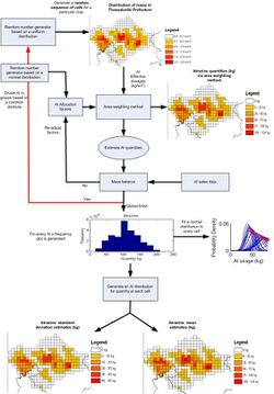
Figure 1 illustrates the procedure.

Starting from a single random grid cell ordering (according to a uniform distribution), for a particular crop, a random weighting (according to a normal distribution) to each set of AIs is multiplied by the AI allocation factors. The allocation factors are multipled by the AI dosages per cultivated crop area (per grid), in order to estimate the AI quantities, based on the area weighting method.

The area weighting method is repeated for all cells for a single random sequence, until the AI quantity from a particular set is depleted (mass balance). Once AI mass is depleted, the allocation factors are normalised according to the remaining AIs. Calculations are repeated until all AI quantities are depleted for a single cell sequence. The same procedure is repeated for a large number of random cell orderings. After the end of the simulations, histograms for each AI (quantity) per cell are generated and suitable distribution functions are fitted, according to known statistical criteria. In this way, AI quantities for all crop cells are presented as a histogram, converted to probability density plots, (as seen in Figure 1.) Once probability density plots have been calculated, estimates of mean AI quantity and standard deviation can be performed, with no guarantee that the AI mass balance is attained.

Spatial allocation of pesticides according to an optimisation function

In this section, it is illustrated how AI quantities could be spatially distributed according to an objective function. Starting with some initial spatial estimates of AI usage (based on the area weighting method), an objective function is formulated, with scope to minimise (or maximise) according to criteria such as:

a) spatial patterns in the geographic activity of pesticides

b) assumed effects of meteorological conditions on pesticide usage

c) level of each AI probability density estimate relative to the maximum probability density of each cell; the weighted sum of all these ratios in a cell is termed the uncertainty index, and the sum of indices in all cells is termed the global uncertainty index.

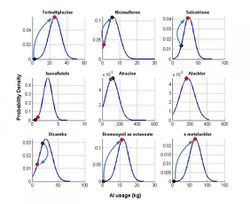
In this example, we illustrate the third approach. Here the objective is to maximise the weighted sum of the AI ratios (initial probability density estimate of the maximum probability density for each AI) present in a cell. Therefore, it is possible to re-allocate all AI quantities from a low probability density to maximum (if applicable) - i.e. quantities with the highest frequency used - ensuring no violation in the total crop cell area (Figure 2).

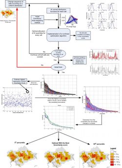
The procedure followed to re-allocate quantities is presented in Figure 3.

Starting from the fitted AI distribution functions for each cell, a large number of random cell realisations are generated (according to a uniform distribution). For each realisation, for each cell, a nonlinear algorithm (trust region reflective algorithm) is implemented. The constraints imposed on the algorithm are on AI quantity and crop area per cell. During the optimisation, if an AI is depleted the objective function changes to exclude that particular AI, and a solution is given for the remaining AIs. Once an optimal solution is found, the next cell in the sequence is processed, until all cells in a prefecture are covered.

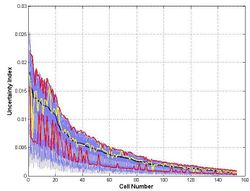
This procedure is repeated for a number of cell realisations, and estimates of the objective function (i.e. uncertainty index) are then sorted in a descending order (in this case, according to the maize crop area, each cell number having a unique ID). In Figure 3, estimates of the objective function are aggregated (to give the global uncertainty index), in order to determine the highest score: AIs closer to the maximum probability density are considered to provide the optimal solution. Figure 4 illustrates variations in the uncertainty index for all cells, where a comparison is made between the optimal solution (yellow line) and results from the area weighting method (initial conditions, black line), together with both confidence intervals (red lines).

Once the best solution for the selected objective function has been identified, the corresponding AI quantities are determined, these are presented in Figure 5, together with the corresponding confidence intervals.

Pesticide maps

The following figures show modelled variations in quantities of Atrazine applied in the Thessaloniki prefecture, according to the methods previously presented.

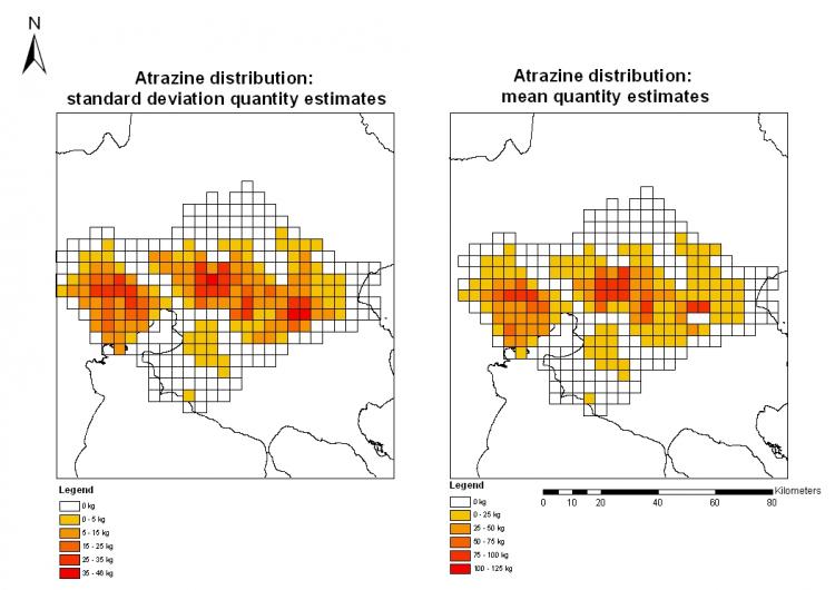Spatial allocation of Atrazine quantity according to the probability functions generated.

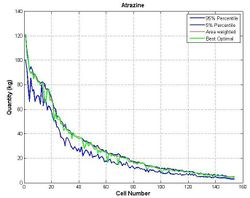
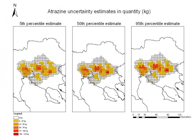Atrazine quantity confidence intervals.