Helsinki energy decision 2015 model
Model with user interface
The final results results can be found from model run 1.11.2015 (token 144638929414). It is the final archived version in English. Objects were stored, so you can download the whole assessment to R in your own computer.
+ Show code- Hide code
# This code is Op_en7237/finalresults on page [[Helsinki energy decision 2015]]
library(OpasnetUtils)
library(ggplot2)
openv.setN(0) # use medians instead of whole sampled distributions
# Download all pre-calculated inputs, e.g. building stock.
objects.latest("Op_en7237", code_name = "intermediates") # [[Helsinki energy decision 2015]]
objects.latest("Op_en6007", code_name = "answer") # [[OpasnetUtils/Drafts]] oggplot
objects.latest("Op_en7392", code_name = "translate") # [[OpasnetUtils/Translate]] translate
objects.latest("Op_en7392", code_name = "dictionary") # [[OpasnetUtils/Translate]] dictionary
BSbase <- 24 # base_size for graph fonts. Use 12 if you use savefig to sav svg fils.
BS <- BSbase
saveobjects <- FALSE
savefigs <- FALSE
language <- "Finnish"
fi <- language == "Finnish"
savefig <- function(
fil,
path = "N:/YMAL/Publications/2015/Helsingin energiapäätös/Kuvat/",
sav = if(exists("savefigs")) savefigs else FALSE,
type = "svg",
height = 18,
width = 24,
units = "cm"
) {
if(sav) {
ggsave(paste(path, fil, ".", type, sep = ""), height = height, width = width, units = units)
}
}
allplants <- c(
'Biofuel heat plants',
'CHP diesel generators',
'Data center heat',
'Deep-drill heat',
'Hanasaari',
'Household air conditioning',
'Household air heat pumps',
'Household geothermal heat',
'Household solar',
'Katri Vala cooling',
'Katri Vala heat',
'Kellosaari back-up plant',
'Loviisa nuclear heat',
'Neste oil refinery heat',
'Salmisaari A&B',
'Salmisaari biofuel renovation',
'Sea heat pump',
'Sea heat pump for cooling',
'Small fuel oil heat plants',
'Small gas heat plants',
'Small-scale wood burning',
'Suvilahti power storage',
'Suvilahti solar',
'Vanhakaupunki museum',
'Vuosaari A',
'Vuosaari B',
'Vuosaari C biofuel',
'Wind mills'
)
shutdown <- allplants[!allplants %in% noshutdown]
shutdown <- c(shutdown, "None")
customdecisions <- data.frame(
Obs = NA,
Decision_maker = "Helen",
Decision = "PlantPolicy",
Option = "Custom",
Variable = c("plantParameters", "energyProcess"),
Cell = c(
paste("Plant:", paste(shutdown, collapse = ","), ";Parameter:Max,Min,Investment cost;Time:>2015", sep = ""),
""
),
Change = c("Replace", "Identity"),
Unit = NA,
Result = 0
)
decisions <- rbind(decisions, customdecisions)
if ("Hanasaari" %in% renovation) {
customdecisions <- data.frame(
Obs = NA,
Decision_maker = "Helen",
Decision = "PlantPolicy",
Option = "Custom",
Variable = rep(c("plantParameters", "energyProcess"), each = 2),
Cell = c(
"Plant:Hanasaari;Time:>=2018;Time:<=2060;Parameter:Max",
"Plant:Hanasaari;Time:>=2018;Parameter:Investment cost",
"Plant:Hanasaari;Fuel:Biofuel;Time:>=2018",
"Plant:Hanasaari;Fuel:Coal;Time:>=2018"
),
Change = rep(c("Replace", "Add"), each = 2),
Unit = NA,
Result = c(640, 100, -0.40, 0.40)
)
decisions <- rbind(decisions, customdecisions)
}
DecisionTableParser(decisions)
oprint(data.frame(
Running = c(
"These plants will be running in the custom plant policy:",
paste(allplants[!allplants %in% shutdown], collapse = ", ")
),
Shutdown = c(
"Plants that will be shut down in the custom plant policy:",
paste(shutdown, collapse = ", ")
)
))
EnergyNetworkDemand <- EvalOutput(EnergyNetworkDemand)
EnergyNetworkDemand@output <- rbind(
EnergyNetworkDemand@output,
data.frame(
Time = rep(c(2025, 2035, 2045, 2055, 2065), each = 4),
EnergySavingPolicy = rep(c("BAU", "Energy saving moderate", "Energy saving total", "WWF energy saving"), times = 5),
Temperature = "(-18,-15]",
EnergyConsumerDemandSource = "Formula",
EnergyConsumerDemandTotalSource = "Formula",
Fuel = "Cooling",
fuelSharesSource = "Formula",
EnergyNetworkDemandResult = 0,
EnergyNetworkDemandSource = "Formula"
)
)
#cat("All energy taxes are assumed zero.\n")
#objects.latest("Op_en4151", code_name = "fuelTax")
#fuelTax <- EvalOutput(fuelTax)
#result(fuelTax) <- 0
fuelUse <- EvalOutput(fuelUse)
fuelUse$Fuel <- factor(
fuelUse$Fuel, levels = c(
"Biofuel",
"Coal",
"Fuel oil",
"Gas",
"Light oil",
"Wood",
"Electricity",
"Electricity_taxed",
"Heat",
"Cooling"
), ordered = TRUE
)
DALY <- EvalOutput(DALYs)
DALYs <- unkeep(DALY, cols = c("Age", "Sex", "Population"))
DALYs <- oapply(DALYs, cols = c("Emission_site", "Emission_height", "Area"), FUN = sum)
DALYs <- DALYs[DALYs$Response == "Total mortality" , ]
EnergyNetworkCost <- EvalOutput(EnergyNetworkCost)
EnergyNetworkCost$Time <- as.numeric(as.character(EnergyNetworkCost$Time))
totalCost <- EvalOutput(totalCost)
totalCost@output$Time <- as.numeric(as.character(totalCost@output$Time))
totalCost <- unkeep(totalCost[totalCost$Time >= 2015 & totalCost$Time <=2065 , ], sources = TRUE)
# Net present value and effective annual cost
discount <- 0.03
times <- c(2015, 2065)
EAC <- EvalOutput(EAC)
if(saveobjects) {
objects.store(list = ls())
cat("All objects stored for later use:\n", paste(ls(), collapse = ", "), "\n")
}
############## POST_PROCESSING AND GRAPHS, VERSION FROM PERFERENCE ANALYSIS
cat(translate("NOTE! In all graphs and tables, the Total energy saving policy is assumed unless otherwise noted\n"))
cat(translate("Total DALYs/a by different combinations of policy options.\n"))
temp <- DALYs[as.character(DALYs$Time) %in% c("2015", "2035") & DALYs$Response == "Total mortality" , ]
oprint(
translate(oapply(temp, INDEX = c("Time", "EnergySavingPolicy", "PlantPolicy"), FUN = sum)),
caption = translate("Table 1: Total DALYs/a by different combinations of policy options."),
caption.placement = "top",
include.rownames = FALSE
)
bui <- oapply(buildings * 1E-6, cols = c("City_area", "buildingsSource"), FUN = sum)
bui <- truncateIndex(bui, cols = "Heating", bins = 4)
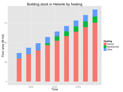
oggplot(bui[bui$EnergySavingPolicy == "BAU" , ], x = "Time", fill = "Heating", binwidth = 5) +
labs(
title = translate("Building stock in Helsinki by heating"),
y = translate("Floor area (M m2)")
)
savefig("Rakennuskannan koko Helsingissä")
oggplot(bui, x = "Time", fill = "Efficiency", binwidth = 5) +
{if(fi) facet_wrap(~ Energiansäästöpolitiikka) else facet_wrap(~ EnergySavingPolicy)} +
labs(
title = translate("Building stock in Helsinki by efficiency policy"),
y = translate("Floor area (M m2)")
)
oggplot(bui, x = "Time", fill = "Renovation", binwidth = 5) +
{if(fi) facet_wrap(~ Energiansäästöpolitiikka) else facet_wrap(~ EnergySavingPolicy)} +
labs(
title = translate("Building stock in Helsinki by renovation policy"),
y = translate("Floor area (M m2)")
)
oggplot(bui[bui$EnergySavingPolicy == "BAU" , ], x = "Time", fill = "Building", binwidth = 5) +
labs(
title = translate("Building stock in Helsinki"),
y = translate("Floor area (M m2)")
)
oggplot(buildings, x = "Time", fill = "Efficiency", binwidth = 5)+
{if(fi) facet_grid(Energiansäästöpolitiikka ~ Korjaukset) else facet_grid(EnergySavingPolicy ~ Renovation)} +
labs(
title = translate("Renovation of buildings by policy and efficiency"),
y = translate("Floor area (M m2)")
)
# Contains also other buildings than district heating and other energy than heating
hea <- EnergyConsumerDemandTotal * temperdays * 24 * 1E-3 # MW -> GWh
hea$Time <- as.numeric(as.character(hea$Time))
temp <- hea[hea$EnergySavingPolicy == "Energy saving total" & !hea$Consumable %in% c("District cooling", "Electric cooling") , ]
oggplot(truncateIndex(temp, cols = "Temperature", bins = 7), x = "Time", fill = "Temperature", binwidth = 5) +
{if(fi) facet_wrap(~ Hyödyke) else facet_wrap(~ Consumable)} +
labs(
title = translate("Energy consumption in all buildings"),
y = translate("Total energy (GWh /a)")
)
temp <- hea[!hea$Consumable %in% c("District cooling", "Electric cooling") , ]
oggplot(temp, x = "Time", fill = "Consumable", binwidth = 5) +
{if(fi) facet_wrap(~ Energiansäästöpolitiikka) else facet_wrap(~ EnergySavingPolicy)} +
labs(
title = translate("Energy consumption in all buildings"),
y = translate("Total energy (GWh /a)")
)
savefig("Helsingin vuotuinen energiantarve")
oggplot(hea, x = "Time", fill = "Consumable", binwidth = 5) +
{if(fi) facet_wrap(~ Energiansäästöpolitiikka) else facet_wrap(~ EnergySavingPolicy)} +
labs(
title = translate("Energy consumption in all buildings"),
y = translate("Total energy (GWh /a)")
)
hea2 <- EnergyNetworkDemand * temperdays * 24 / 1000 # MW -> GWh
hea2$Time <- as.numeric(as.character(hea2$Time))
oggplot(hea2, x = "Time", fill = "Fuel", binwidth = 5) +
{if(fi) facet_wrap(~ Energiansäästöpolitiikka) else facet_wrap(~ EnergySavingPolicy)} +
labs(
title = translate("Energy demand in the network"),
fill = translate("Consumable"),
y = translate("Total energy (GWh /a)")
)
savefig("Energiankulutus verkossa Helsingissä")
eb <-EnergyNetworkOptim[EnergyNetworkOptim$Process_variable_type == "Activity",]
eb <- eb[eb$EnergySavingPolicy == "Energy saving total" , ]
colnames(eb@output)[colnames(eb@output) == "Process_variable_name"] <- "Plant"
eb$Process_variable_type <- NULL
ebtemp <- eb[eb$Time %in% c("2035") & eb$PlantPolicy == "BAU" & eb$Temperature != "(-18,-15]" , ]
ebtemp <- truncateIndex(ebtemp, cols = "Plant", bins = 7)
oggplot(ebtemp, x = "Temperature", fill = "Plant", turnx = TRUE) +
labs(
title = translate("Power plant activity by temperature daily optim \nPlant policy = BAU, Year = 2035"),
x = translate("Temperature of the day"),
y = translate("Average daily activity (MW)")
)
ebtemp <- eb[eb$Time %in% c("2035") & eb$Temperature != "(-18,-15]" , ]
ebtemp <- truncateIndex(ebtemp, cols = "Plant", bins = 10)
oggplot(ebtemp, x = "Temperature", fill = "Plant", turnx = TRUE) +
{if(fi) facet_wrap(~ Voimalapolitiikka) else facet_wrap(~ PlantPolicy)} +
labs(
title = translate("Power plant activity by temperature daily optim in 2035"),
x = translate("Temperature of the day"),
y = translate("Average daily activity (MW)")
)
savefig("Helsingin päivittäinen kaukolämpötase")
ebtemp <- eb[eb$Time %in% c("2005") & eb$PlantPolicy == "BAU" & eb$Temperature == "(0,3]" , ]
ebtemp <- truncateIndex(ebtemp, cols = "Plant", bins = 10)
oggplot(ebtemp, x = "Plant", fill = "Plant", turnx = TRUE) +
{if(fi) facet_wrap(~ Lämpötila) else facet_wrap( ~ Temperature)} +
theme(axis.text.x = element_blank()) + # Turn text and adjust to right
labs(
title = translate("Power plant activity by temperature daily optim \nPlant policy = BAU, Year = 2005"),
y = translate("Average daily activity (MW)")
)
fu <- fuelUse / 3.6E+6 # From MJ/a -> GWh/a
fu <- fu[fu$EnergySavingPolicy == "Energy saving total" , ]
fu$Burner <- NULL
fu$Time <- as.numeric(as.character(fu$Time))
futemp <- fu[fu$Time %in% c("2015", "2035", "2065") & fu$PlantPolicy == "BAU" , ]
futemp <- truncateIndex(futemp, cols = "Plant", bins = 7) * -1
oggplot(futemp, x = "Fuel", fill = "Plant", turnx = TRUE) +
{if(fi) facet_grid(Aika ~ Energiansäästöpolitiikka) else facet_grid(Time ~ EnergySavingPolicy)} +
labs(
title = translate("Energy commodity flows \n Plant policy = BAU"),
y = translate("Total annual energy (GWh/a)")
)
futemp <- fu[fu$Time %in% c("2005") & fu$PlantPolicy == "BAU" , ]
futemp <- truncateIndex(futemp, cols = "Plant", bins = 7) * -1
oggplot(futemp, x = "Fuel", fill = "Plant", turnx = TRUE) +
labs(
title = translate("Energy commodity flows in 2005 \n Plant policy = BAU"),
y = translate("Total annual energy (GWh/a)")
)
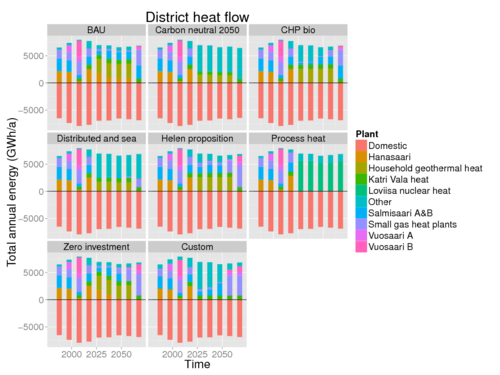
futemp <- fu[fu$Fuel %in% c("Heat") , ]
futemp <- truncateIndex(futemp, cols = "Plant", bins = 10) * -1
oggplot(futemp,
x = "Time", fill = "Plant", binwidth = 5) +
{if(fi) facet_wrap(~ Voimalapolitiikka) else facet_wrap(~ PlantPolicy)} +
labs(
title = translate("District heat flow"),
y = translate("Total annual energy (GWh/a)")
)
savefig("Helsingin vuotuinen kaukolämpötase")
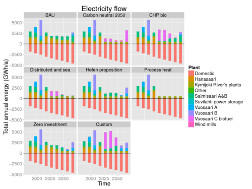
futemp <- fu[fu$Fuel %in% c("Electricity") & fu$Plant != "Kymijoki River's plants", ]
futemp <- truncateIndex(futemp, cols = "Plant", bins = 7) * -1
# Does not contain plants outside Helsinki: Kymijoki River's plants, a share of Olkiluoto nuclear plant.
oggplot(futemp, x = "Time", fill = "Plant", binwidth = 5) +
{if(fi) facet_wrap(~ Voimalapolitiikka) else facet_wrap(~ PlantPolicy)} +
labs(
title = translate("Electricity flow"),
y = translate("Total annual energy (GWh/a)")
)
savefig("Helsingin vuotuinen sähkötase")
emis <- truncateIndex(emissions, cols = "Emission_site", bins = 5)
emis <- emis[emis$EnergySavingPolicy == "Energy saving total" & emis$Fuel != "Electricity" , ]
levels(emis$Fuel)[levels(emis$Fuel) == "Electricity_taxed"] <- "Electricity bought"
emis$Time <- as.numeric(as.character(emis$Time))
oggplot(emis, x = "Time", fill = "Fuel", binwidth = 5) +
{if(fi) facet_grid(Saaste ~ Voimalapolitiikka, scale = "free_y") else facet_grid(Pollutant ~ PlantPolicy, scale = "free_y")} +
labs(
title = translate("Emissions from heating in Helsinki"),
y = translate("Emissions (ton /a)")
) +
scale_x_continuous(breaks = c(2000, 2050))
savefig("Helsingin energiantuotannon päästöt")
da <- DALYs[DALYs$EnergySavingPolicy == "Energy saving total" & DALYs$Fuel != "Electricity" , ]
levels(da$Fuel)[levels(da$Fuel) == "Electricity_taxed"] <- "Electricity bought"
da$Time <- as.numeric(as.character(da$Time))
oggplot(da, x = "Time", fill = "Fuel", binwidth = 5) +
{if(fi) facet_wrap(~ Voimalapolitiikka) else facet_wrap(~ PlantPolicy)} +
labs(
title = translate("Health effects of PM2.5 from heating in Helsinki"),
y = translate("Health effects (DALY /a)")
)
savefig("Helsingin energiantuotannon terveysvaikutukset")
fp <- fuelPrice[fuelPrice$Fuel %in% c(
"Biofuel",
"Coal",
"Electricity_taxed",
"Fuel oil",
"Heat",
"Light oil",
"Natural gas",
"Peat"
) , ]
fp$Time <- as.numeric(as.character(fp$Time))
levels(fp$Fuel)[levels(fp$Fuel) == "Electricity_taxed"] <- "Electricity"
ggplot(translate(fp@output), if(fi) {
aes(x = Aika, y = fuelPriceResult, colour = Polttoaine, group = Polttoaine)
} else {
aes(x = Time, y = fuelPriceResult, colour = Fuel, group = Fuel)
}) +
geom_line(size = 2)+theme_gray(base_size = BS) +
labs(
title = translate("Fuel prices (with tax)"),
y = translate("Price (Eur/MWh)")
)
savefig("Polttoaineiden verolliset hinnat")
tc <- truncateIndex(totalCost, cols = "Plant", bins = 11) / 10 * -1 # Yearly benefits (costs are negative)
tc <- tc[tc$EnergySavingPolicy == "Energy saving total" , ]
oggplot(tc, x = "Time", fill = "Cost", binwidth = 10) +
{if(fi) facet_wrap(~ Voimalapolitiikka) else facet_wrap( ~ PlantPolicy)} +
labs(
y = translate("Yearly cash flow (Meur)"),
title = translate("Total benefits and costs of energy production")
)+
scale_x_continuous(breaks = c(2000, 2020, 2040, 2060))
savefig("Energiantuotannon kokonaiskustannus Helsingissä kustannuksittain")
oggplot(tc, x = "Time", fill = "Plant", binwidth = 10) +
{if(fi) facet_wrap(~ Voimalapolitiikka) else facet_wrap(~ PlantPolicy)} +
labs(
y = translate("Yearly cash flow (Meur)"),
title = translate("Total benefits and costs of energy production")
)+
scale_x_continuous(breaks = c(2000, 2020, 2040, 2060))
savefig("Energiantuotannon kokonaiskustannus Helsingissä voimaloittain")
eac <- EAC[EAC$EnergySavingPolicy == "Energy saving total" , ] * -1
BS <- BSbase * 0.7 # Plot the next two graphs with smaller font because they are busy graphs.
eac2 <- eac[!eac$Plant %in% c(
'Household air conditioning',
'Household solar',
'Katri Vala cooling',
'Kellosaari back-up plant',
'Sea heat pump for cooling',
'Small-scale wood burning',
'Suvilahti power storage',
'Suvilahti solar',
'Vanhakaupunki museum',
'Wind mills'
) , ]
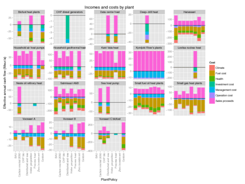
oggplot(eac2, x = "PlantPolicy", fill = "Cost", turnx = TRUE) +
{if(fi) facet_wrap(~ Voimala, scale = "free_y") else facet_wrap(~ Plant, scale = "free_y")} +
labs(
title = translate("Incomes and costs by plant"),
y = translate("Effective annual cash flow (Meur/a)")
)
savefig("Helsingin voimalaitosten kustannustehokkuus")
oggplot(eac2, x = "PlantPolicy", fill = "Cost", turnx = TRUE)+
{if(fi) facet_wrap(~ Voimala) else facet_wrap(~ Plant)} +
labs(
title = translate("Incomes and costs by plant"),
y = translate("Effective annual cash flow (Meur/a)")
)
savefig("Helsingin voimalaitosten kustannustehokkuus yhtenäisasteikolla")
BS <- BSbase
eac <- truncateIndex(eac, cols = "Plant", bins = 11)
oggplot(eac, x = "PlantPolicy", fill = "Plant", turnx = TRUE)+
labs(
title = translate("Incomes and costs by plant policy"),
y = translate("Effective annual cash flow (Meur/a)")
)
oggplot(eac, x = "PlantPolicy", fill = "Cost", turnx = TRUE)+
labs(
title = translate("Incomes and costs by plant policy"),
y = translate("Effective annual cash flow (Meur/a)")
)
savefig("Teholliset tulot ja menot energiantuotannosta Helsingissä kustannuksittain")
temp <- truncateIndex(plantParameters[plantParameters$Parameter == "Max" , ], cols = "Plant", bins = 11)
temp <- temp[temp$Time >= 2000 & temp$Time <=2070 , ]
oggplot(temp, x = "Time", fill = "Plant", binwidth = 1) +
{if(fi) facet_wrap(~ Voimalapolitiikka) else facet_wrap(~ PlantPolicy)} +
labs(
title = translate("Energy production capacity by plant policy"),
y = translate("Maximum capacity (MW)")
)
savefig("Energiantuotantokapasiteetin kehitys Helsingissä")
# odag() #Plots a directed acyclic graph of ovariables used in the model.
# This causes an internal error, so it must be the last row of the model.
| |
Rationale
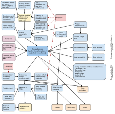
Causal diagram for the assessment.
Case-specific ovariables
Name is the name of ovariable that has case-specific rather than default content. Ident is the indentifier of the code that defines the case-specific ovariable. Token is the same as Ident but it uses a specific version of the code rather than the newest version. Latest is the code for an ovariable whose dependencies will be changed, i.e. who has the case-specific ovariable as parent. Get is the same as Latest but a specific version rather than the newest version is fetched.
Case-specific ovariables(-)| Obs | Name | Ident | Token | Latest | Get | Description |
|---|
| 1 | buildings | Op_en6289/buildingstest | | Op_en5488/EnergyConsumerDemand | | [[Building model]] buildings # Generic building model |
| 2 | changeBuildings | Op_en7115/changeBuildings | | Op_en6289/buildingstest | | |
| 3 | demolitionRate | Op_en7115/demolitionRate | | Op_en6289/buildingstest | | |
| 4 | efficiencyShares | Op_en5488/efficiencyShares | | Op_en6289/buildingstest | | |
| 5 | emissionLocations | Op_en7311/emissionLocationsPerPlant | | Op_en2791/emissionstest | | [[Helsinki energy production]] emissionLocations, used by[[Emission factors for burning processes]] emissions |
| 6 | energyProcess | Op_en7311/energyProcess | | Op_en5141/EnergyNetworkOptim | | [[Helsinki energy production]] energyProcess, used by [[Energy balance]] EnergyConsumerDemandTotal |
| 7 | exposure | Op_en5813/exposure | | | | [[Intake fractions of PM]] exposure # uses Humbert iF as default. |
| 8 | fuelShares | Op_en7311/fuelShares | | Op_en2791/emissionFactors | | [[Helsinki energy production]] fuelShares, used by ([[Emission factors for burning processes]] emissionFactors?) |
| 9 | plantParameters | Op_en7311/plantParameters | | Op_en3283/totalCost | | [[Helsinki energy production]] plantParameters, used by [[Economic impacts]] plantCost |
| 10 | renovationRate | Op_en7115/renovationRate | | Op_en6289/buildingstest | | [[Building stock in Helsinki]] renovationRate |
| 11 | | | | Op_en7115/renovationRate | | [[Building stock in Helsinki]] renovationRate case-specific adjustment in formula |
| 12 | renovationShares | Op_en7115/renovationShares | | Op_en6289/buildingstest | | |
| 13 | stockBuildings | Op_en7115/stockBuildings | | Op_en6289/buildingstest | | |
| 14 | temperatures | Op_en2959/temperatures | | Op_en5488/EnergyConsumerDemand | | [[Outdoor air temperature in Finland]], used by [[Energy use of buildings]] EnergyConsumerDemand |
| 15 | temperdays | Op_en2959/temperatures | | Op_en5488/EnergyConsumerDemand | | [[Outdoor air temperature in Finland]] |
Calculations
+ Show code- Hide code
## This code is Op_en7237/intermediates on page [[Helsinki energy decision 2015]]
library(OpasnetUtils)
library(ggplot2)
library(rgdal)
#library(maptools)
library(RColorBrewer)
#library(classInt)
#library(RgoogleMaps)

### Technical parameters

openv.setN(0) # use medians instead of whole sampled distributions
BS <- 24 # base_size = font size in graphs
figstofile <- FALSE
saveobjects <- TRUE

########################## Case-specific data and submodels

### Decisions
decisions <- opbase.data("Op_en7237", subset = "Decisions") # [[Helsinki energy decision 2015]]

oprint(decisions)

### Energy production in Helsinki

objects.latest("Op_en6007", code_name = "answer") # [[OpasnetUtils/Drafts]] findrest
objects.latest("Op_en7311", code_name = "energyProcess") # [[Helsinki energy production]]
objects.latest("Op_en7311", code_name = "plantParameters") # [[Helsinki energy production]]
objects.latest("Op_en4151", code_name = "fuelPrice") # [[Prices of fuels in heat production]]

objects.latest("Op_en5141", code_name = "EnergyNetworkOptim") # [[Energy balance]] incl EnergyNetworkCost

### Building data in Helsinki

# Observation years must be defined for an assessment.
obstime <- Ovariable("obstime", data = data.frame(Obsyear = factor(seq(1985, 2065, 10), ordered = TRUE), Result = 1))
heatingShares <- 1 # Shares of different heating types in the building stock (already in the building data)
heating_before <- FALSE # Should heatingShares be calculated before renovate and timepoints (or after)?
efficiency_before <- TRUE # Should efficiencyShares be calculated before renovate and timepoints (or after)?

objects.latest("Op_en7115", code_name = "stockBuildings") # [[Building stock in Helsinki]]
objects.latest("Op_en7115", code_name = "changeBuildings") # [[Building stock in Helsinki]]
objects.latest("Op_en7115", code_name = "demolitionRate") # [[Building stock in Helsinki]]
objects.latest("Op_en7115", code_name = "renovationRate") # [[Building stock in Helsinki]]
objects.latest("Op_en7115", code_name = "renovationShares") # [[Building stock in Helsinki]]
objects.latest("Op_en5488", code_name = "efficiencyShares") # [[Energy use of buildings]]

objects.latest("Op_en6289", code_name = "buildingstest") # [[Building model]] # Generic building model.

## Energy use
#objects.latest("Op_en5488", code_name = "energyUseTemperature")        # [[Energy use of buildings]] temperature version of energyUse
objects.latest("Op_en5488", code_name = "temperene")        # [[Energy use of buildings]] temperature version of energyUse
objects.latest("Op_en5488", code_name = "nontemperene")        # [[Energy use of buildings]] temperature version of energyUse
objects.latest("Op_en2959", code_name = "temperatures") # [[Outdoor air temperature in Finland]]
#objects.latest("Op_en5488", code_name = "energyUseTemperature") # [[Energy use of buildings]]
objects.latest("Op_en5488", code_name = "EnergyConsumerDemand") # [[Energy use of buildings]]

requiredName <- "Heat" # Name of the fuel type that must match for input and output

### Energy and emissions
objects.latest("Op_en7311", code_name = "emissionLocationsPerPlant") # [[Helsinki energy production]] also heatingShares
objects.latest("Op_en2791", code_name = "emissionFactors") # [[Emission factors for burning processes]]
objects.latest("Op_en2791", code_name = "emissionstest") # [[Emission factors for burning processes]]
objects.latest("Op_en7311", code_name = "fuelShares") # [[Helsinki energy production]]
objects.latest("Op_en7311", code_name = "nondynsupply") # [[Helsinki energy production]]
timelylimit <- 10000 # The largest production (MW) available at each plant (used to describe time-varying limits).

## Exposure

objects.latest("Op_en5813", code_name = "exposure") # [[Intake fractions of PM]] uses Humbert iF as default.

## Health assessment

objects.latest('Op_en2261', code_name = 'totcases') # [[Health impact assessment]] totcases and dependencies.
objects.latest('Op_en5461', code_name = 'DALYs') # [[Climate change policies and health in Kuopio]] DALYs, DW, L

population <- 623732 # Contains only the Helsinki city, i.e. assumes no exposure outside city. (Wikipedia)
# Note: the population size does NOT affect the health impact if the exposure-response function in linear.
# However, it DOES affect exposure estimates.

# DALYshortcut is for a quicker health impact calculations, as it directly uses the Helsinki conditions.

objects.latest("Op_en7237", code_name = "DALYshortcut") # [[Helsinki energy decision 2015]]

objects.latest("Op_en7379", code_name = "externalities") # [[External cost]]
objects.latest("Op_en3283", code_name = "totalCost") # [[Economic impacts]]
objects.latest("Op_en3283", code_name = "EAC") # [[Economic impacts]]

################################# Actual model and some intermediate processing.

DecisionTableParser(decisions)

# Remove previous decisions, if any.

forgetDecisions()

renovationRate <- EvalOutput(renovationRate) * 10 # Rates for 10-year periods

buildings <- EvalOutput(buildings)

buildings$EnergySavingPolicy <- factor(
		buildings$EnergySavingPolicy,
		levels = c("BAU", "Energy saving moderate", "Energy saving total", "WWF energy saving"),
		ordered = TRUE
)

EnergyConsumerDemand <- EvalOutput(EnergyConsumerDemand)

EnergyNetworkDemand <- EvalOutput(EnergyNetworkDemand)

EnergyNetworkDemand@output <- rbind(
	EnergyNetworkDemand@output,
	data.frame(
		Time = rep(c(2025, 2035, 2045, 2055, 2065), each = 4),
		EnergySavingPolicy = rep(c("BAU", "Energy saving moderate", "Energy saving total", "WWF energy saving"), times = 5),
		Temperature = "(-18,-15]",
		EnergyConsumerDemandSource = "Formula",
		EnergyConsumerDemandTotalSource = "Formula",
		Fuel = "Cooling",
		fuelSharesSource = "Formula",
		EnergyNetworkDemandResult = 0,
		EnergyNetworkDemandSource = "Formula"
	)
)

########################### SAVE OBJECTS

if(saveobjects) {

	# Clean decisions and previous results not wanted/needed by the half-model

	energyProcess@output <- data.frame()
	plantParameters@output <- data.frame()
	EnergyNetworkOptim@output <- data.frame()
	#EnergyConsumerDemand@output <- data.frame()

	totcases@output <- data.frame()
	DALYs@output <- data.frame()
	exposure@output <- data.frame()
	rm(saveobjects, dictionary) # Remove technical objects that may be updated independently of the model

	objects.store(list = ls()) # Save all objects of the global environment.
	cat("All objects stored for later use:\n", paste(ls(), collapse = ", "), "\n")
}

############################ Output tables and graphs
if(FALSE) {

fuelUse <- EvalOutput(fuelUse)

fuelUse$Fuel <- factor(
	fuelUse$Fuel, levels = c(
		"Biofuel",
		"Coal",
		"Fuel oil",
		"Gas",
		"Light oil",
		"Wood",
		"Electricity",
		"Electricity_taxed",
		"Heat",
		"Cooling"
	), ordered = TRUE
)

# Calculate exposure based on average iF.
exposure <- EvalOutput(exposure)
exposure <- exposure[exposure$Area == "Average" , ]
exposure <- oapply(exposure, cols = c("Plant", "Emission_site", "Emission_height", "Area"), FUN = sum)
totcases <- EvalOutput(totcases)
DALYs <- EvalOutput(DALYs)
EnergyNetworkCost <- EvalOutput(EnergyNetworkCost)

cat("Total DALYs/a by different combinations of policy options.\n")

temp <- DALYs[as.character(DALYs$Time) %in% c("2015", "2035", "2065") & DALYs$Response == "Total mortality" , ]

oprint(
		oapply(temp, INDEX = c("Time", "EnergySavingPolicy", "PlantPolicy"), FUN = sum),
		caption = "Table 1: Total DALYs/a by different combinations of policy options.",
		caption.placement = "top",
		include.rownames = FALSE
)

####################### Post-processing and graphs

bui <- oapply(buildings * 1E-6, cols = c("City_area", "buildingsSource"), FUN = sum)
bui <- truncateIndex(bui, cols = "Heating", bins = 4)

oggplot(bui[bui$EnergySavingPolicy == "BAU" , ], x = "Time", fill = "Heating", binwidth = 5) +
		labs(
				title = "Building stock in Helsinki by heating",
				y = "Floor area (M m2)"
		)

oggplot(bui, x = "Time", fill = "Efficiency", binwidth = 5) +
		facet_grid(. ~ EnergySavingPolicy) +
		labs(
				title = "Building stock in Helsinki by efficiency policy",
				y = "Floor area (M m2)"
		)

oggplot(bui, x = "Time", fill = "Renovation", binwidth = 5) +
		facet_grid(. ~ EnergySavingPolicy) +
		labs(
				title = "Building stock in Helsinki by renovation policy",
				y = "Floor area (M m2)"
		)

oggplot(bui[bui$EnergySavingPolicy == "BAU" , ], x = "Time", fill = "Building", binwidth = 5) +
		labs(
				title = "Building stock in Helsinki",
				y = "Floor area (M m2)"
		)

oggplot(buildings, x = "Time", fill = "Efficiency", binwidth = 5)+
		facet_grid(EnergySavingPolicy ~ Renovation) +
		labs(
				title = "Renovation of buildings by policy and efficiency",
				y = "Floor area (M m2)"
		)

emissions$Time <- as.numeric(as.character(emissions$Time))

# Plot energy need and emissions

hea <- EnergyConsumerDemand * temperdays * 24 * 1E-9 # From W -> GWh /a.
hea <- hea[hea$Consumable == "Heating" , ]
hea <- oapply(hea, cols = c("City_area", "buildingsSource"), FUN = sum)
hea <- truncateIndex(hea, cols = "Heating", bins = 4)

oggplot(hea, x = "Time", fill = "Renovation", binwidth = 5) +
		facet_wrap( ~ EnergySavingPolicy) +
		labs(
				title = "Energy used in heating in Helsinki",
				x = "Time",
				y = "Heating energy (GWh /a)"
		)

eb <-EnergyNetworkOptim[EnergyNetworkOptim$Process_variable_type == "Activity",]
colnames(eb@output)[colnames(eb@output) == "Process_variable_name"] <- "Plant"
eb$Process_variable_type <- NULL

ebtemp <- eb[eb$Time %in% c("2035") & eb$EnergySavingPolicy == "BAU" & eb$PlantPolicy == "BAU" , ]
ebtemp <- truncateIndex(ebtemp, cols = "Plant", bins = 7)

oggplot(ebtemp, x = "Plant", fill = "Plant") + facet_wrap( ~ Temperature) +
		theme(axis.text.x = element_blank()) + # Turn text and adjust to right
		labs(
				title = "Power plant activity by temperature daily optim \nPlant policy = BAU, Year = 2035",
				y = "Power output daily average (MW)"
		)

fu <- fuelUse
fu$Burner <- NULL
fu <- fu / 3.6E+6 # From MJ/a -> GWh/a
fu$Time <- as.numeric(as.character(fu$Time))

futemp <- fu[fu$Time %in% c("2015", "2035", "2065") & fu$PlantPolicy == "BAU" , ]
futemp <- truncateIndex(futemp, cols = "Plant", bins = 7) * -1
oggplot(futemp, x = "Fuel", fill = "Plant", turnx = TRUE) + facet_grid(Time ~ EnergySavingPolicy) +
		labs(
				title = "Energy commodity flows \n Plant policy = BAU",
				y = "Total annual energy (GWh/a)"
		)

futemp <- fu[fu$Fuel %in% c("Heat") , ]
futemp <- truncateIndex(futemp, cols = "Plant", bins = 10) * -1
oggplot(futemp, x = "Time", fill = "Plant", binwidth = 5) + facet_grid(EnergySavingPolicy ~ PlantPolicy) +
		labs(
				title = "District heat flow",
				y = "Total annual energy (GWh/a)"
		)

futemp <- fu[fu$Fuel %in% c("Electricity") , ]
futemp <- truncateIndex(futemp, cols = "Plant", bins = 10) * -1
oggplot(futemp, x = "Time", fill = "Plant", binwidth = 5) + facet_grid(EnergySavingPolicy ~ PlantPolicy) +
		labs(
				title = "Electricity flow",
				y = "Total annual energy (GWh/a)"
		)

oggplot(emissions[emissions$EnergySavingPolicy == "BAU" , ], x = "Time", fill = "Fuel", binwidth = 5) +
		facet_grid(Pollutant ~ PlantPolicy, scale = "free_y") +
		labs(
				title = "Emissions from heating in Helsinki",
				x = "Time (Energy saving policy = BAU)",
				y = "Emissions (ton /a)"
		)

oggplot(exposure[exposure$Exposure_agent == "PM2.5" , ], x = "Time", fill = "Fuel", binwidth = 5) +
		facet_grid(EnergySavingPolicy ~ PlantPolicy) +
		labs(
				title = "Exposure to PM2.5 from heating in Helsinki",
				x = "Time",
				y = "Average PM2.5 (µg/m3)"
		)

oggplot(DALYs, x = "Time", fill = "Fuel", binwidth = 5) + facet_grid(EnergySavingPolicy ~ PlantPolicy) +
		labs(
				title = "Health effects in DALYs of PM2.5 from heating in Helsinki",
				y = "Health effects (DALY /a)"
		)
} # END if(FALSE)
| |
Building stock in Helsinki
Question
What is the building stock in Helsinki and its projected future?
Answer
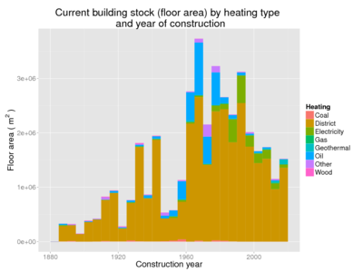
Current building stock in Helsinki by heating type.
Projected building stock based on 2015 data and urban plans.
Rationale
This part contains the data needed for calculations about the building stock in Helsinki. It shows the different building and heating types in Helsinki, and how much and what kind of renovations are done for the existing building stock in a year, including how much and how old building stock is demolished. This data is used in further calculations in the model.
There is also some other important data that wasn't used in the model's calculations. These include more accurate renovation statistics for residential buildings, U-value changes for renovations and thermal transmittance of different parts of residential buildings. This data is found under Data not used.
Carbon neutral Helsinki 2035
Building stock
These tables are based on FACTA database classifications and their interpretation for assessments.
This data is used for modelling. The data is large and can be seen from the Opasnet Base. Technical parts on this page are hidden for readability. Building types should match Energy use of buildings#Baseline energy consumption.
| Show details
|
Building types(-)| Obs | Building types in Facta | Building | Number of the class |
|---|
| 1 | Yhden asunnon talot | Detached and semi-detached houses | 11 | | 2 | Kahden asunnon talot | Detached and semi-detached houses | 12 | | 3 | Muut erilliset pientalot | Detached and semi-detached houses | 13 | | 4 | Rivitalot | Attached houses | 21 | | 5 | Ketjutalot | Attached houses | 22 | | 6 | Luhtitalot | Blocks of flats | 32 | | 7 | Muut asuinkerrostalot | Blocks of flats | 39 | | 8 | Vapaa-ajan asuinrakennukset | Free-time residential buildings | 41 | | 9 | Myymälähallit | Commercial | 111 | | 10 | Liike- ja tavaratalot, kauppakeskukset | Commercial | 112 | | 11 | Myymälärakennukset | Commercial | 119 | | 12 | Hotellit, motellit, matkustajakodit, kylpylähotellit | Commercial | 121 | | 13 | Loma-, lepo- ja virkistyskodit | Commercial | 123 | | 14 | Vuokrattavat lomamökit ja osakkeet (liiketoiminnallisesti) | Commercial | 124 | | 15 | Muut majoitusliikerakennukset | Commercial | 129 | | 16 | Asuntolat, vanhusten palvelutalot, asuntolahotellit | Commercial | 131 | | 17 | Muut asuntolarakennukset | Commercial | 139 | | 18 | Ravintolat, ruokalat ja baarit | Commercial | 141 | | 19 | Toimistorakennukset | Offices | 15 | | 20 | Toimistorakennukset | Offices | 151 | | 21 | Rautatie- ja linja-autoasemat, lento- ja satamaterminaalit | Transport and communications buildings | 161 | | 22 | Kulkuneuvojen suoja- ja huoltorakennukset | Transport and communications buildings | 162 | | 23 | Pysäköintitalot | Transport and communications buildings | 163 | | 24 | Tietoliikenteen rakennukset | Transport and communications buildings | 164 | | 25 | Muut liikenteen rakennukset | Transport and communications buildings | 169 | | 26 | Keskussairaalat | Buildings for institutional care | 211 | | 27 | Muut sairaalat | Buildings for institutional care | 213 | | 28 | Terveyskeskukset | Buildings for institutional care | 214 | | 29 | Terveydenhuollon erityislaitokset | Buildings for institutional care | 215 | | 30 | Muut terveydenhuoltorakennukset | Buildings for institutional care | 219 | | 31 | Vanhainkodit | Buildings for institutional care | 221 | | 32 | Lasten- ja koulukodit | Buildings for institutional care | 222 | | 33 | Kehitysvammaisten hoitolaitokset | Buildings for institutional care | 223 | | 34 | Muut huoltolaitosrakennukset | Buildings for institutional care | 229 | | 35 | Lasten päiväkodit | Buildings for institutional care | 231 | | 36 | Muualla luokittelemattomat sosiaalitoimen rakennukset | Buildings for institutional care | 239 | | 37 | Vankilat | Buildings for institutional care | 241 | | 38 | Teatterit, konsertti- ja kongressitalot, oopperat | Assembly buildings | 311 | | 39 | Elokuvateatterit | Assembly buildings | 312 | | 40 | Kirjastot ja arkistot | Assembly buildings | 322 | | 41 | Museot ja taidegalleriat | Assembly buildings | 323 | | 42 | Näyttelyhallit | Assembly buildings | 324 | | 43 | Seurain-, nuoriso- yms. talot | Assembly buildings | 331 | | 44 | Kirkot, kappelit, luostarit, rukoushuoneet | Assembly buildings | 341 | | 45 | Seurakuntatalot | Assembly buildings | 342 | | 46 | Muut uskonnollisten yhteisöjen rakennukset | Assembly buildings | 349 | | 47 | Jäähallit | Assembly buildings | 351 | | 48 | Uimahallit | Assembly buildings | 352 | | 49 | Tennis-, squash- ja sulkapallohallit | Assembly buildings | 353 | | 50 | Monitoimihallit ja muut urheiluhallit | Assembly buildings | 354 | | 51 | Muut urheilu- ja kuntoilurakennukset | Assembly buildings | 359 | | 52 | Muut kokoontumisrakennukset | Assembly buildings | 369 | | 53 | Peruskoulut, lukiot ja muut | Educational buildings | 511 | | 54 | Ammatillisten oppilaitosten rakennukset | Educational buildings | 521 | | 55 | Korkeakoulurakennukset | Educational buildings | 531 | | 56 | Tutkimuslaitosrakennukset | Educational buildings | 532 | | 57 | Järjestöjen, liittojen, työnantajien yms. opetusrakennukset | Educational buildings | 541 | | 58 | Muualla luokittelemattomat opetusrakennukset | Educational buildings | 549 | | 59 | Voimalaitosrakennukset | Industrial buildings | 611 | | 60 | Yhdyskuntatekniikan rakennukset | Industrial buildings | 613 | | 61 | Teollisuushallit | Industrial buildings | 691 | | 62 | Teollisuus- ja pienteollisuustalot | Industrial buildings | 692 | | 63 | Muut teollisuuden tuotantorakennukset | Industrial buildings | 699 | | 64 | Teollisuusvarastot | Warehouses | 711 | | 65 | Kauppavarastot | Warehouses | 712 | | 66 | Muut varastorakennukset | Warehouses | 719 | | 67 | Paloasemat | Fire fighting and rescue service buildings | 721 | | 68 | Väestönsuojat | Fire fighting and rescue service buildings | 722 | | 69 | Muut palo- ja pelastustoimen rakennukset | Fire fighting and rescue service buildings | 729 | | 70 | Navetat, sikalat, kanalat yms. | Agricultural buildings | 811 | | 71 | Eläinsuojat, ravihevostallit, maneesit | Agricultural buildings | 819 | | 72 | Viljankuivaamot ja viljan säilytysrakennukset | Agricultural buildings | 891 | | 73 | Kasvihuoneet | Agricultural buildings | 892 | | 74 | Turkistarhat | Agricultural buildings | 893 | | 75 | Muut maa-, metsä- ja kalatalouden rakennukset | Agricultural buildings | 899 | | 76 | Saunarakennukset | Other buildings | 931 | | 77 | Talousrakennukset | Other buildings | 941 | | 78 | Muualla luokittelemattomat rakennukset | Other buildings | 999 | | 79 | Ammatilliset oppilaitokset | Educational buildings | | | 80 | Kirjastot | Other buildings | | | 81 | Lastenkodit, koulukodit | Other buildings | | | 82 | Loma- lepo- ja virkistyskodit | Other buildings | | | 83 | Monitoimi- ja muut urheiluhallit | Other buildings | | | 84 | Museot, taidegalleriat | Assembly buildings | | | 85 | Muut kerrostalot | Blocks of flats | | | 86 | Muut majoitusrakennukset | Commercial | | | 87 | Muut terveydenhoitorakennukset | Buildings for institutional care | | | 88 | Terveydenhoidon erityislaitokset (mm. kuntoutuslaitokset) | Buildings for institutional care | | | 89 | Vapaa-ajan asunnot | Free-time residential buildings | | | 90 | Viljankuivaamot ja viljan säilytysrakennukset, siilot | Warehouses | |
----#: . Viimeiset 12 riviä (ilman numeroa) ovat tyyppejä jotka ovat datassa (tai ainakin vanhassa taulukossa) mutta puuttuvat Sonjan luokittelusta. --Jouni (talk) 12:57, 24 August 2015 (UTC) (type: truth; paradigms: science: comment)
For residential buildings (classes A and B) the classification is kept more detailed than for other buildings. This is because residential buildings are the biggest energy consumers in Helsinki and different classes of residential buildings are examined separately.
Reference for the classification: http://www.stat.fi/meta/luokitukset/rakennus/001-1994/koko_luokitus.html
Heating types(-)| Obs | Heating types in Facta | Heating |
|---|
| 1 | | Other | | 2 | Kauko- tai aluelämpö | District heating | | 3 | Kevyt polttoöljy | Light oil | | 4 | Kivihiili, koksi tms. | Coal | | 5 | Maalämpö tms. | Geothermal | | 6 | Puu | Wood | | 7 | Raskas polttoöljy | Fuel oil | | 8 | Sähkö | Electricity | | 9 | Kaasu | Gas | | 10 | Muu | Other |
The structures of the tables are based on CyPT Excel file N:\YMAL\Projects\ilmastotiekartta\Helsinki Data Input Template - Building Data.xlsx.
|
+ Show code- Hide code
library(OpasnetUtils)
library(ggplot2)

# [[Building stock in Helsinki]], building stock, locations by city area (in A Finnish coordinate system)
#stockBuildings <- Ovariable("stockBuildings", ddata = "Op_en7115.stock_details")
#colnames(stockBuildings@data)[colnames(stockBuildings@data) == "Built"] <- "Time"
#colnames(stockBuildings@data)[colnames(stockBuildings@data) == "Postal code"] <- "City_area"

# [[Building stock in Helsinki]]
dat <- opbase.data("Op_en7115.stock_details")[ , c(
#	"Rakennus ID",
	"Sijainti",
	"Valmistumisaika",
#	"Julkisivumateriaali",
	"Käyttötarkoitus",
#	"Lämmitystapa",
	"Polttoaine",
#	"Rakennusaine",
#	"Varusteena koneellinen ilmanvaihto",
#	"Perusparannus",
#	"Kunta rakennuttajana",
#	"Energiatehokkuusluokka",
#	"Varusteena aurinkopaneeli",
	"Tilavuus",
	"Kokonaisala",
	"Result" # Kerrosala m2
)]

colnames(dat) <- c("City_area", "Time", "Building types in Facta", "Heating types in Facta", "Tilavuus", "Kokonaisala", "Kerrosala")
dat$Time <- as.numeric(substring(dat$Time, nchar(as.character(dat$Time)) - 3))

#dat <- dat[dat$Time != 2015 , ] # This is used to compare numbers to 2014 statistics.

dat$Time <- as.numeric(as.character((cut(dat$Time, breaks = c(0, 1885 + 0:26*5), labels = as.character(1885 + 0:26*5)))))
dat$Tilavuus <- as.numeric(as.character(dat$Tilavuus))
dat$Kokonaisala <- as.numeric(as.character(dat$Kokonaisala))
dat$Kerrosala <- as.numeric(as.character(dat$Kerrosala))

build <- tidy(opbase.data("Op_en7115.building_types"))
colnames(build)[colnames(build) == "Result"] <- "Building"

heat <- tidy(opbase.data("Op_en7115.heating_types"))
colnames(heat)[colnames(heat) == "Result"] <- "Heating"

######################
# Korjaus
########################
temp <- as.character(heat$Heating)
temp[temp == "District heating"]  <- "District"
temp[temp == "Light oil"]  <- "Oil"
temp[temp == "Fuel oil"]  <- "Oil"

heat$Heating <- temp
########################################

dat <- merge(merge(dat, build), heat)#[c("City_area", "Time", "Building", "Heating", "stockBuildingsResult")]

dat$Kerrosala[is.na(dat$Kerrosala)] <- dat$Kokonaisala[is.na(dat$Kerrosala)] * 0.8 # If floor area is missing, estimate from total area.

cat("Kerrosala ilman 2015 (m^2)\n")
oprint(aggregate(dat["Kerrosala"], by = dat["Building"], FUN = sum, na.rm = TRUE))
cat("Kokonaisala ilman 2015 (m^2)\n")
oprint(aggregate(dat["Kokonaisala"], by = dat["Building"], FUN = sum, na.rm = TRUE))
cat("Tilavuus ilman 2015 (m^3)\n")
oprint(aggregate(dat["Tilavuus"], by = dat["Building"], FUN = sum, na.rm = TRUE))

temp <- aggregate(dat["Kerrosala"], by = dat[c("Time", "Building", "Heating")], FUN =sum, na.rm = TRUE)
colnames(temp)[colnames(temp) == "Kerrosala"] <- "stockBuildingsResult"

stockBuildings <- Ovariable("stockBuildings", data = temp)

objects.store(stockBuildings)
cat("Ovariable stockBuildings stored.\n")
| |
Construction and demolition
It is assumed that construction occurs at a constant rate so that there is an increase of 42% in 2050 compared to 2013. Energy efficiency comes from Energy use of buildings.
Fraction of houses demolished per year.
Heating type conversion
The fraction of heating types in the building stock reflects the situation at the moment of construction and not currently. The heating type conversion corrects this by changing a fraction of heating methods to a different one at different timepoints. Cumulative fraction, other timepoints will be interpolated.
Renovations
Estimates from Laura Perez and Stephan Trüeb, unibas.ch N:\YMAL\Projects\Urgenche\WP9 Basel\Energy_scenarios_Basel_update.docx
Fraction of houses renovated per year(%)| Obs | Age | Result | Description |
|---|
| 1 | 0 | 0 | Estimates from Laura Perez and Stephan Trüeb |
| 2 | 20 | 0 | Assumption Result applies to buildings older than the value in the Age column. |
| 3 | 25 | 1 | |
| 4 | 30 | 1 | |
| 5 | 50 | 1 | |
| 6 | 100 | 1 | |
| 7 | 1000 | 1 | |
Building model
Question
How to estimate the size of the building stock of a city, including heating properties, renovations etc? The situation is followed over time, and different policies can be implemented.
Answer
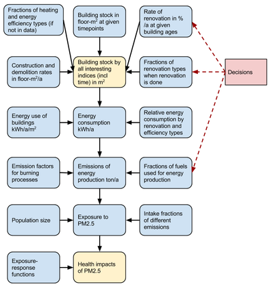
Causal diagram of the
building model. The actual model is up to the yellow node Building stock, and the rest is an example how the result can be used in models downstream.
The building model follows the development of a city's or area's building stock over time. The output of the model is the floor area (or volume, depending on the input data) of the building stock of a city at specified timepoints, classified by energy efficiency, heating type, and optionally by other case-specific characteristics. The model functions as part of Opasnet's modeling environment and it is coded using R. It uses specific R objects called ovariables. The model can also be downloaded and run on one's own computer.
The model is given data about the building stock of a certain city or area during a certain period of time. The data can be described with very different levels of precision depending on the situation and what kind of information is needed. Some kind of data on the energy efficiency and heating type is necessary, but even rough estimates suffice. Then again, if there is sufficient data, the model can analyse even individual buildings.
In addition to that, the model can describe changes in the building stock, i.e. construction of new buildings and demolishing
of old ones. Data on the heating- and energy efficiencies of new and demolished buildings is required at the same level of precision as that of other buildings. This data is used to calculate how construction and demolishing change the building stock's size and heating types.
The model takes into account the energy renovation of existing buildings. They are analysed using two variables:
firstly, what fraction of the building stock is energy renovated yearly and secondly, what type of renovation it is.
This information, too, can be rough or precise and detailed. It can describe the whole building stock with a single number or be
specific data on the time, the building's age, use or other background information.
- For examples of model use, see Helsinki energy decision 2015, Building stock in Kuopio and Climate change policies and health in Kuopio.
The overall equation in the model is this:

- B = buildings, floor area of buildings in specified groups
- Bs = stockBuildings, floor area of the current buildings
- Bc = changeBuildings, floor area of constructed and demolished (as negative areas) buildings
- Hs = heatingShares, fractions of different heating types in a group of buildings
- Es = efficiencyShares, fractions of different efficiency classes in a group of buildings
- Rr = renovationRate, fraction of buildings renovated per year
- Rs = renovationShares, fractions of different renovation types performed when buildings are renovated
- O = obstime, timepoints for which the building stock is calculated.
- Indices required (also other indices are possible)
- t = Obsyear, time of observation. This is renamed Time on the output data.
- c = Construction year (the index is named 'Time' in the input data), time when the building was built.
- a = Age, age of building at a timepoint. This is calculated as a = t - b.
- h = Heating, primary heating type of a building
- e = Efficiency, efficiency class of building when built
- r = Renovation, type of renovation done to a non-renovated building (currently, you can only renovate a building once)
The model is iterative across the Obsyear index so that renovations performed at one timepoint are inherited to the next timepoint, and that situation is the starting point for renovations in that timepoint.
Rationale
Inputs and calculations
Variables in the building model
| Variable |
Measure |
Indices |
Missing data
|
| stockBuildings (case-specific data from the user) e.g. Building stock in Helsinki or Building stock in Kuopio
|
Amount of building stock (typically in floor-m2) at given timepoints.
|
Required indices: Time (time the building was built. If not known, present year can be used for all buildings.) Typical indices: City_area, Building (building type)
|
You must give either stockBuildings, heatingShares, and efficiencyShares or changeBuildings or both. For missing data, use 0.
|
| heatingShares (case-specific data from the user)
|
Fractions of heating types. Should sum up to 1 within each group defined by optional indices.
|
Required indices: Heating. Typical indices: Time, Building
|
If no data, use 1 as a placeholder.
|
| efficiencyShares (case-specific data from the user)
|
Fraction of energy efficiency types. Should sum up to 1 for each group defined by other indices.
|
Required indices: Efficiency. Typical indices: Time, Building.
|
If no data, use 1 as default.
|
| changeBuildings (case-specific data from the user)
|
Construction or demolition rate as floor-m2 at given timepoints.
|
Required indices: Obsyear, Time, Efficiency, Heating. If both stockBuildings and changeBuildings are used, changeBuildings should have all indices in stockBuildings, heatingShares, and efficiencyShares. Typical indices: Building, City_area.
|
If the data is only in stockBuildings, use 0 here.
|
| renovationShares (case-specific data from the user)
|
Fraction of renovation types when renovation is done. Should sum to 1 for each group defined by other indices.
|
Required indices: Renovation, Obsyear. Obsyear is the time when the renovation is done
|
If no data, use 1 as default.
|
| renovationRate (case-specific data from user. You can also use fairly generic data from Building stock in Helsinki or Building stock in Kuopio.)
|
Rate of renovation (fraction per time unit).
|
Required indices: Age (the time difference between construction and renovation, i.e. Obsyear - Time for each building).
|
If no data, use 0.
|
| obstime (assessment-specific years of interest)
|
The years to be used in output. The only index Obsyear contains the years to look at; Result is 1.
|
Required indices: Obsyear. Typical indices: other indices are not allowed.
|
-
|
This code defines the generic building model object called buildings. Other objects needed can be found from case-specific pages, see table above.
+ Show code- Hide code
### This code is Op_en6289/buildingstest on page [[Building model]].

library(OpasnetUtils)

########## Calculate all building events (constructions, demolitions, renovations)

buildings <- Ovariable("buildings",
	dependencies = data.frame(Name = c(
		"stockBuildings",
		"changeBuildings",
		"heatingShares", # This can be indexed by building year (Time) or Observation year (Obsyear)
		"efficiencyShares", # Same here
		"renovationShares",
		"renovationRate", # Fraction of buildings renovated between timepoints
		"demolitionRate", # Fraction of buildings demolished between timepoints
		#"heatTypeConversion", # Is dependent on buil, which defined in the formula (must handle withihn formula). Fraction of heating types converted to other
		"obstime" # In the new version obstime is ovariable with column Obsyear.
	)),
	formula = function(...) {

		stock <- stockBuildings * obstime
		if( ! "Efficiency" %in% colnames(stock@output)) { # Add those shares that are missing
			stock <- stock * efficiencyShares
		}
		if( ! "Heating" %in% colnames(stock@output)) {
			stock <- stock * heatingShares
		}

		stock2 <- changeBuildings * obstime
		if( ! "Efficiency" %in% colnames(stock2@output)) { # Add those shares that are missing
			stock2 <- stock2 * efficiencyShares
		}
		if( ! "Heating" %in% colnames(stock2@output)) {
			stock2 <- stock2 * heatingShares
		}

		stock2@output$Time <- as.factor(stock2@output$Time) # Also stock@output$Time is factor
		buil <- OpasnetUtils::combine(stock, stock2) # Buildings in the whole timeline
		buil <- unkeep(buil, sources = TRUE)
		buil@output$Age <- as.numeric(as.character(buil@output$Obsyear)) - as.numeric(as.character(buil@output$Time))
		buil@marginal <- c(buil@marginal, TRUE)
		buil@output <- buil@output[buil@output$Age >= 0 , ]

		# Note that if stockBuildings and changeBuildings have different marginals (typically policies),
		# there will be NA in these indices. This will be corrected below.
		for(i in colnames(buil@output)[buil@marginal]) {
			if(any(is.na(buil@output[[i]]))) {
				buil@output <- fillna(buil@output, i)
				print(paste("Column", i, "treated with fillna (difference between stockBuildings and changeBuildings)."))
			}
		}

		# heatTypeConversion dependent on buil, which defined above, and hence must be handled here.
		# Scope is messed up due to the dependency and the following produces error when run within EvalOutput of buildings
		#objects.latest("Op_en7115", code_name = "heatTypeConversion")
		#heatTypeConversion <- EvalOutput(heatTypeConversion)
		heatTypeConversion <- function(){
			dat <- opbase.data("Op_en7115", subset = "Yearly_heating_converted_factor")
			colnames(dat)[colnames(dat) == "Time"] <- "Obsyear"

			dat$Obs <- NULL

			out <- data.frame()
			temp <- unique(dat[c("Heating_from", "Heating_to")])
			for (i in 1:nrow(temp)) {
				onetype <- merge(temp[i,], dat)
				tempout <- merge(obstime@output, onetype, all.x = TRUE)[c("Obsyear","Result")]
				tempout <- merge(tempout, temp[i,])

				for (j in (1:nrow(tempout))[is.na(tempout$Result)]) {
					a <- onetype$Obsyear[which.min(abs(as.numeric(as.character(onetype$Obsyear)) - as.numeric(as.character(obstime$Obsyear[j]))))]
					tempout$Result[j] <- onetype$Result[a]
				}
				out <- rbind(out, tempout)
			}

			out <- Ovariable(output = out, marginal = colnames(out) != "Result")

			colnames(out@output)[colnames(out@output) == "Heating_from"] <- "Heating"

			out <- buil * out

			out1 <- out
			out1$Result <- - out1$Result
			out1$Heating_to <- NULL

			out$Heating <- out$Heating_to
			out$Heating_to <- NULL

			out@output <- rbind(out1@output, out@output)
			heatTypeConversion <- out
			return(out)
		}
		buil <- OpasnetUtils::combine(buil, heatTypeConversion())

		temp1 <- merge(renovationRate, unique(buil@output["Age"])) # Avoid redundant calculations
		temp1@name <- renovationRate@name
		temp2 <- renovationShares
		temp2@output <- temp2@output[temp2@output$Renovation == "None" , ]
		renovate <- (1 - temp1) * (1 - temp2) # Assumes that data has row for Renovation: None = 0
		renovate <- OpasnetUtils::combine(renovate, temp1 * renovationShares)

		out <- data.frame()
		prevreno <- unkeep(buil * renovate * 0, sources = TRUE) # Previously renovated buildings for the first time point
		prevreno@output <- prevreno@output[prevreno@output$Renovation != "None" , ][1,] # Just take one renovated example row
		marginals <- colnames(prevreno@output)[prevreno@marginal]
		demolitionRate <- unkeep(demolitionRate, sources = TRUE) # Would otherwise cause trouble in rbind.

		for(i in obstime@output$Obsyear) { # Accumulate the building stock
			# Take the building stock
			temp <- buil
			temp@output <- temp@output[temp@output$Obsyear == i , ] # Take buildings of year i
			prevreno@output$Obsyear <- i # update the observation year of the previous renovation

			# Remove from the stock buildings that are demolished
			temp <- temp * (1 - demolitionRate)

			# Subtrack from the building stock buildings that are already renovated.
			temp <- OpasnetUtils::combine(temp, -1 * oapply(prevreno, cols = "Renovation", FUN = sum)) # Subtract previously renovated
			reno <- unkeep(temp * renovate, sources = TRUE) # Renovate the current non-renovated stock
			# If renovate does not match with this timepoint, mark all buildings here as unrenovated.
			# Is there new renovation in this time point?
			if(sum(result(reno)) == 0) {
				reno <- temp * Ovariable(
					output = data.frame(Renovation = "None", Result = 1),
					marginal = c(TRUE, FALSE)
				)
			}
			newreno <- OpasnetUtils::combine(prevreno, reno) # Renovated buildings in this time point.
			# Take the previous timepoints, and previously renovated and now possibly renovated together.
			out <- rbind(newreno@output, out) # Add previously and now renovated together
			prevreno <- unkeep(newreno, sources = TRUE)
			prevreno@output <- prevreno@output[prevreno@output$Renovation != "None" , ]
		}
		out <- Ovariable(output = out, marginal = colnames(out) %in% marginals)

		# Note that if buil and renovate have different marginals (typically policies),
		# there will be NA in these indices. This will be corrected below.
		for(i in colnames(out@output)[out@marginal]) {
			if(any(is.na(out@output[[i]]))) {
				out@output <- fillna(out@output, i)
				print(paste("Column", i, "treated with fillna (difference between buil and renovate)."))
			}
		}

		out <- oapply(unkeep(out, sources = TRUE), cols = c("Age", "Time"), FUN = sum)
		colnames(out@output)[colnames(out@output) == "Obsyear"] <- "Time" # From now on, Time means the time of observation
		out@output$Time <- as.numeric(as.character(out@output$Time))

		return(out)
	}
)

objects.store(buildings)

cat("Saved ovariable buildings\n")
| |
Energy use of buildings
Question
How to model the use of energy of buildings based on either annual consumption per floor area, or energy efficiency per floor area per indoor-outdoor temperature difference?
Answer
An example code for fetching and using the variables.
Rationale
Input
Variables needed to calculate the EnergyConsumerDemand. Note that there are several different methods available, and temperature data is not needed in an annual energy version.
| Dependencies |
Measure |
Indices |
Missing data
|
| buildings (from the model).
|
Floor area of the building stock to be heated
|
Typical indices: Building, Heating, Efficiency, Renovation
|
You can use value 1 to calculate energy need per 1 m2 floor area.
|
| temperene (fairly generic data for a given cultural and climatic area, e.g. from Energy use of buildings)
|
Energy need per floor area and indoor-outdoor temperature difference (W /m2 /K)
|
Required indices: Consumable, Fuel (Commodity). Typical indices: Building, Heating.
|
if this data is missing, you can only calculate building stock but nothing further.
|
| nontemperene (fairly generic data for a given cultural and climatic area, e.g. from Energy use of buildings)
|
Energy need for hot water and other non-temperature-dependent activities
|
Required indices: Consumable, Fuel (Commodity).
|
Use 0 to calculate energy demand excluding non-heating energy use.
|
| temperatures (location-specific data)
|
Average outdoor temperatures for particular temperature bins.
|
Reuired indices: Temperature.
|
If missing, use the annual energy version.
|
| temperdays (location-specific data)
|
Number of days per year for particular temperature bins.
|
Required indices: Temperature.
|
If missing, use the annual energy version.
|
| efficiencyRatio (fairly generic data for a cultural and climatic area, e.g. from Energy use of buildings)
|
Relative energy consumption compared with the efficiency group Old.
|
Required indices: Efficiency. Typical indices: Time, Building.
|
If no data, use 1 as default.
|
| renovationRatio (fairly generic data for a cultural and climatic area, e.g. from Energy use of buildings)
|
Relative energy consumption compared with the Renovation location None.
|
Required indices: Renovation. Typical indices: Building.
|
If no data, use 1 as default.
|
Temperature-dependent calculations
The code below assumes energy consumption factors relative to floor area (W /m2 /K). Local temperature data must be given in either individual or aggregated way. Individual way has temperature data for all timepoints (e.g. days or hours) of the given year, and heatingTime = 1. Aggregated way has a specific Temperature index (e.g. very cold, cold, cool etc) in both ovariables temperature and heatingTime. The ovariable temperature tells what is the actual temperature when it is "very cold", and heatingTime tells how many hours it is "very cold" during the year.

where
- Q = Energy used for heating and cooling (kWh /a)
- B = floor area of a building stock indexed by renovation and efficiency (m2)
- U = energy consumption factor per floor area for a building type (W /m2 /K)
- T = temperature outside (assumes that no heating is needed if outside temperature is 17 degrees Celsius)
- E = relative efficiency of a building stock based on energy class when built (no unit)
- R = relative efficiency of a building stock based on energy class after renovated (no unit)
- W = heating need of hot water (W)
- t = time spent in a particular outdoor temperature (h /a)
- indices used:
- b = building type
- e = efficiency class of building
- r = renovation class of building
- t = ambient temperature class
Baseline energy consumption
Heat reflects the energy need for heating in situations where the outdoor temperature is below 17 °C. Cooling reflects the cooling need (measured as thermal energy, not electricity!) in situations where the outdoor temperature is above 24 °C. This is not a U value, because it is about energy use per floor area, not about heat loss through building structures per m2. For estimating temperene, we take the total energy consumption in Helsinki and divide that with the total floor area and average temperature difference, see Helsinki energy consumption#U values based on overall data.
Energy use per area and temperature difference(W /K /m2)| Obs | Consumable | Fuel | Energy flow | Description |
|---|
| 1 | Heating | Heat | 1.66 | See Helsinki energy consumption: 6921.65/24/365/38990000/(17-4.8)*1E+9 |
| 2 | District cooling | Cooling | 0.3 | Guesswork. This uses centralised system. |
| 3 | Electric cooling | Electricity | 0.3 | Guesswork. This uses apartment-specific appliances. |
Temperature-independent energy consumption per floor area.
Temperature-independent energy use per area(W /m2)| Obs | Consumable | Fuel | Energy intensity | Description |
|---|
| 1 | Consumer electricity | Electricity | 5 | Assumes 50 kWh /m2 /a (see below) |
| 2 | Hot water | Heat | 4 | Assumes that hot water is ca. 20 % of energy need of heating: 6921.65/24/365/38990000*1E+9*0.2 |
Energy efficiency in heating
What is the relative energy consumption of different efficiency classes compared with Old? This table tells that with some background information about heat (in kWh/m2/a), electricity, and water consumption.
Energy use by energy class of building(ratio)| Obs | Efficiency | Ratio | Heat | User electricity | Water | Description |
|---|
| 1 | Traditional | 1.2-1.4 | 200 | | | Guesstimate |
| 2 | Old | 1 | 150 | | 30 | Pöyry 2011 s.28 |
| 3 | New | 0.4-0.5 | 70 | 50 | 40 | Pöyry 2011 s.32 (2010 SRMK) |
| 4 | Low-energy | 0.2-0.25 | 35 | 50 | 40 | Personal communication |
| 5 | Passive | 0.1-0.16 | 17.5 - 25 | 50 | 40 | Pöyry 2011 s.33; Personal communication |
Energy efficiency of buildings when they are built(%)| Obs | Efficiency | Constructed | Fraction | Description |
|---|
| 1 | Traditional | 1800-1944 | 100 | |
| 2 | Old | 1945-1994 | 100 | |
| 3 | New | 1995-2019 | 100 | |
| 4 | New | 2020-2029 | 10-20 | |
| 5 | Low-energy | 2020-2029 | | The rest of energy class |
| 6 | Passive | 2020-2029 | 25-35 | |
| 7 | New | 2030-2039 | 5-10 | |
| 8 | Low-energy | 2030-2039 | 20-50 | |
| 9 | Passive | 2030-2039 | | The rest of energy class |
| 10 | New | 2040-2070 | 0-5 | |
| 11 | Low-energy | 2040-2070 | 10-30 | |
| 12 | Passive | 2040-2070 | | The rest of energy class |
- Old: old buildings to be renovated (or in need of renovation)
- New: normal new buildings (no current need of renovation)
- Low-energy: buildings consuming about half of the energy of a new building
- Passive: buildings consuming a quarter or less of the energy of a new building
- Chinese green building system: [2] [3]
Impact of renovations
Energy saving potential of different renovations(ratio,kWh/m2/a)| Obs | Renovation | Relative | Absolute | Renovation details | Description |
|---|
| 1 | Windows | 0.85 | 25 | New windows and doors | Pöyry 2011 |
| 2 | Technical systems | 0.50 | 75 | New windows, sealing of building's sheath, improvement of building's technical systems | Pöyry 2011 |
| 3 | Sheath reform | 0.35 | 100 | New windows, sealing of building's sheath, improvement of building's technical systems, significant reform of building's sheath | Pöyry 2011 |
| 4 | General | 0.85 | - | General renovation | Pöyry 2011 |
| 5 | None | 1 | 0 | Renovation not done | |
Helsinki energy consumption
Question
How much energy is consumed and to what purposes in Helsinki?
Answer
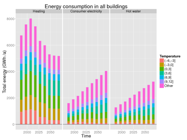
Energy consumed for heating, cooling, hot water, and consumer electricity in Helsinki. Note: the future consumption is based on
Energy saving total scenario from the assessment
Helsinki energy decision 2015, not business-as-usual.
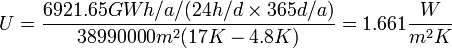
There is no answer code here, because the U value 1.661 W /m2 /K is directly used in Energy use of buildings#Baseline energy consumption.
Rationale
U values based on overall data
The total heat consumption by district-heated buildings is 6921.65 GWh in 2013 (see below). We can derive the total energy efficiency value expressed as W /m2 /K for floor area and temperature difference between indoors and outdoors. The typical energy efficiency calculations (using the so called U value) assume that outdoor 17 °C is thermoneutral and lower values require heating. The total floor area of district-heated buildings is 38990000 m2 in 2015 according to the Helsinki energy decision 2015 model. The annual average temperature in Helsinki is 4.8 °C [4] and during heating season Sep-May 1.4 C (Opasnet data). Therefore the energy efficiency value (approximate U value) is
Energy consumption statistics
Total energy consumption in Helsinki in 2013 (GWh) [1]
| |
Adjusted for temperature |
Not adjusted for temperature
|
| District heating |
6921.65 |
6461.00
|
| Separate heating |
303.89 |
284.01
|
| Electric heating |
339.23 |
316.65
|
| Consumer electricity |
3988.10 |
3988.10
|
| Private cars |
1294.06 |
1294.06
|
| Other road traffic |
794.33 |
794.33
|
| Trains |
111.16 |
111.16
|
| Ships |
432.12 |
432.12
|
| Industry and machinery |
147.60 |
147.60
|
| Total |
14332.14 |
13829.03
|
Helsinki energy production
Question
What is the amount of energy produced (including distributed production) in Helsinki? Where is it produced (-> emissions)? Which processes are used in its production?
Answer
This code is used to fetch the ovariables on this page for modelling.
Rationale
This page contains data about the heat plants in Helsinki. It tells, how much and what type of energy a plant produces per unit of fuel, how much the plants cost and the locations of the power plant emissions. This data is then further used in the model.
Amount produced is determined largely by the energy balance in Helsinki and Helsinki energy consumption. The maximum energy produced and fuels used by of all Helen's power plants can be found here: https://www.helen.fi/kotitalouksille/neuvoa-ja-tietoa/tietoa-meista/energiantuotanto/voimalaitokset/
Energy processes
Heat, power and cooling processes(MJ /MJ)| Obs | Plant | Burner | Electricity | Electricity_taxed | Heat | Cooling | Coal | Gas | Fuel oil | Biofuel | Description |
|---|
| 1 | Biofuel heat plants | Large fluidized bed | 0 | 0 | 0.85-0.91 | 0 | 0 | 0 | 0 | -1 | |
| 2 | CHP diesel generators | Diesel engine | 0.3 | 0 | 0.3-0.5 | 0 | 0 | 0 | -1 | 0 | Efficiency not known well in practice |
| 3 | Data center heat | None | 0 | -0.27 - -0.23 | 1 | 0 | 0 | 0 | 0 | 0 | Same as Neste without transport of heat |
| 4 | Deep-drill heat | None | 0 | -0.4 - -0.1 | 1 | 0 | 0 | 0 | 0 | 0 | Experimental technology |
| 5 | Hanasaari | Large fluidized bed | 0.31 | 0 | 0.60 | 0 | -1 | 0 | 0 | 0 | Assume 91 % efficiency. Capacity: electricity 220 MW heat 420 MW Loss 64 MW |
| 6 | Household air heat pumps | None | 0 | -0.7 - -0.2 | 1 | 0 | 0 | 0 | 0 | 0 | The efficiency of heat pumps is largely dependent on outside air temperature, it's feasible for a household air heat pump to reach COP 5 at 10 °C and COP 1.5 at -25 °C. |
| 7 | Household air conditioning | None | 0 | -0.7 - -0.2 | 0 | 1 | 0 | 0 | 0 | 0 | |
| 8 | Household geothermal heat | None | 0 | -0.36 - -0.31 | 1 | 0 | 0 | 0 | 0 | 0 | Motiva 2014 |
| 9 | Katri Vala cooling | None | 0 | -0.36 - -0.31 | 0 | 1 | 0 | 0 | 0 | 0 | District cooling produced by absorption (?) heat pumps. Same as heat pumps for heating, Motiva 2014. |
| 10 | Katri Vala heat | None | 0 | -0.36 - -0.31 | 1 | 0 | 0 | 0 | 0 | 0 | Heat from cleaned waste water and district heating network's returning water. Motiva 2014 |
| 11 | Kellosaari back-up plant | Large fluidized bed | 0.3 - 0.5 | 0 | 0 | 0 | 0 | 0 | -1 | 0 | Only produces electric power |
| 12 | Kymijoki River's plants | None | 1 | 0 | 0 | 0 | 0 | 0 | 0 | 0 | Hydropower |
| 13 | Loviisa nuclear heat | None | 0 | -0.4 - -0.1 | 1 | 0 | 0 | 0 | 0 | 0 | Assumes that for each MWh heat produced, 0.1-0.2 MWh electricity is lost in either production or when heat is pumped to Helsinki. |
| 14 | Neste oil refinery heat | None | 0 | -0.31 - -0.27 | 1 | 0 | 0 | 0 | 0 | 0 | Motiva 2014 |
| 15 | Salmisaari A&B | Large fluidized bed | 0.32 | 0 | 0.59 | 0 | -1 | 0 | 0 | 0 | Capacity: electricity 160 MW heat 300 MW loss 46 MW |
| 16 | Sea heat pump | None | 0 | -0.36 - -0.31 | 1 | 0 | 0 | 0 | 0 | 0 | Motiva 2014 |
| 17 | Sea heat pump for cooling | None | 0 | -0.36 - -0.31 | 0 | 1 | 0 | 0 | 0 | 0 | Assuming the same as for heating |
| 18 | Small-scale wood burning | Household | 0 | 0 | 0.5 - 0.9 | 0 | 0 | 0 | 0 | -1 | |
| 19 | Small gas heat plants | Large fluidized bed | 0 | 0 | 0.91 | 0 | 0 | -1 | 0 | 0 | |
| 20 | Small fuel oil heat plants | Large fluidized bed | 0 | 0 | 0.91 | 0 | 0 | 0 | -1 | 0 | |
| 21 | Suvilahti power storage | None | 1 | 0 | 0 | 0 | 0 | 0 | 0 | 0 | |
| 22 | Suvilahti solar | None | 1 | 0 | 0 | 0 | 0 | 0 | 0 | 0 | |
| 23 | Vanhakaupunki museum | None | 1 | 0 | 0 | 0 | 0 | 0 | 0 | 0 | Hydropower |
| 24 | Vuosaari A | Large fluidized bed | 0.455 | 0 | 0.455 | 0 | 0 | -1 | 0 | 0 | Capacity: electricity 160 MW heat 160 MW loss 30 MW |
| 25 | Vuosaari B | Large fluidized bed | 0.5 | 0 | 0.41 | 0 | 0 | -1 | 0 | 0 | Capacity: electricity 500 MW heat 424 MW loss 90 MW |
| 26 | Vuosaari C biofuel | Large fluidized bed | 0.47 | 0 | 0.44 | 0 | 0 | 0 | 0 | -1 | |
| 27 | Wind mills | None | 1 | 0 | 0 | 0 | 0 | 0 | 0 | 0 | |
Notes about the data in the table:
- Household air heat pumps data from heat pump comparison[2]
- Household geothermal heat data from Energy Department of the United States: Geothermal Heat Pumps[3]
- Small-scale wood burning data from Energy Department of the United States: Wood and Pellet Heating[4]
- Loss of thermal energy through distribution is around 10 %. From Norwegian Water Resources and Energy Directorate: Energy in Norway.[5]
- Sustainable Energy Technology at Work: Use of waste heat from refining industry, Sweden.[6]
- Chalmers University of Technology: Towards a Sustainable Oil Refinery, Pre-study for larger co-operation projects[7]
- CHP diesel generators are regular diesel generators, but they are located in apartment houses and operated centrally. This way, it is possible to produce electricity when needed and use the excess heat, instead of district heat, to warm up the hot water of the house.
- Motiva estimates for heat pumps processes and costs for heating:[8]
- Mechanical heat pumps usually have COP (coefficient of performance, thermal output energy per electric input energy needed) is 2.5 - 7.5.
- In district heating, mechanical heat pumps have typically COP around 3.
- Absorption heat pumps have COP typically 1.5 - 1.8. They do not use much electricity but they need either hot water or steam to operate. Therefore, they are not suitable for producing district heat from warm water with temperatures in the range of 25 - 30 °C (Neste) or 10-15 °C (sea heat).
- The report uses these values for energy prices (€/MWh): bought electricity 50, process steam 25, wood chip 20, district heating 40, own excess heat 0.
- The investment cost of a heat pump system (ominaiskustannus) in the cases described in this report were 0.47-0.73 M€/MWth for mechanical heat pumps and 0.072 - 0.102 M€/MWth for absorption heat pumps. These values do not include the pipelines needed, which may vary a lot; in these cases the pipeline costs were 0.1 - 2.5 times the cost of the heat pump.
- The energy efficiency is theoretically COP = Tout / (Tout - Tin), and the actual COP values are typically 65 - 75 % of that. If we assume that we want 95 °C district heat out, we get
- for sea heat pumps: COP = 368 K / (368 K - 283 K) = 4.3 ideally and in practice 2.8 - 3.2. Electricity needed per 1 MWh output: 0.31 - 0.36 MWh.
- Neste process heat: COP = 368 K / (368 K - 303 K) = 5.7 ideally and in practice 3.7 - 4.2. Electricity needed per 1 MWh output: 0.23 - 0.27 MWh (plus what is needed for pumping the heat for 25 km, say + 0.04 MWh)
Plant specifications
These equations below aim to reflect the energy production facilities and capabilities. The min and max values tell about the range of energy production of the plant, and the cost values tell the costs of building and running the powerplant.
Note! Maintenance cost only contains costs that do not depend on activity. Operational cost contains costs that depend on activity but NOT fuel price; those are calculated separately based on energy produced.
Plant parameters(MW,MW,M€,M€ /a,€ /MWh)| Obs | Years_active | Plant | Min | Max | Investment cost | Management cost | Operation cost | Description |
|---|
| 1 | 2017-2070 | Biofuel heat plants | 0 | 100-300 | 360 | 10 | 4-12 | biofuels (pellets, wood chips and possibly biochar) |
| 2 | 2025-2070 | CHP diesel generators | 0 | 1441 | 144 | 1 | 1 | Assuming all of Helsinki's apartment houses were fitted with 100 kW generators. |
| 3 | 2025-2080 | Deep-drill heat | 0 | 300 | 300-900 | 9.6 | 40 | Investment cost from ETSAP |
| 4 | 1965-2040 | Hanasaari | 0 | 640 | 0 | 9.6 | 8 | 95% coal, 5% pellets. Assume cost of running and maintenance in coal plants 15€/kW (Sähköenergian kustannusrakenne) |
| 5 | 2010-2060 | Household air heat pumps | 0 | 112 | 200-300 | 10 | 5 | Assuming all of Helsinki's detached and row houses were fitted with air heat pumps |
| 6 | 2010-2060 | Household air conditioning | 0 | 67 | 150-200 | 10 | 5 | |
| 7 | 2016-2060 | Household geothermal heat | 0 | 335 | 380-450 | 10 | 5 | Assuming all of Helsinki's detached and row houses were fitted with geothermal heat pumps |
| 8 | 2020-2035 | Household solar | 0 | 105 | 220-250 | 5 | 5 | Assuming 700000 m2 suitable for solar panels. |
| 9 | 2010-2070 | Katri Vala cooling | 0 | 60 | 0 | 10 | 3 | waste water. Max from Helen |
| 10 | 2005-2065 | Katri Vala heat | 0 | 90 | 0 | 10 | 3 | waste water. Max from Helen |
| 11 | 1980-2050 | Kellosaari back-up plant | 0 | 120 | 0 | 10 | 20 | oil |
| 12 | 1980-2070 | Kymijoki River's plants | 0 | 60 | 0 | 10 | 1-4 | hydropower |
| 13 | 2022-2080 | Loviisa nuclear heat | 0 | 1800-2600 | 400-4000 | 10 | 5 | Investment cost includes energy tunnel (double of Neste) but NOT building cost of plant. Some estimate for typical district heat pipes on ground is 2 M€/km; this is clearly a minimum for this project. |
| 14 | 2020-2060 | Neste oil refinery heat | 0 | 300 | 200-500 | 10 | 5 | |
| 15 | 1975-2050 | Salmisaari A&B | 0 | 506 | 0 | 7.6 | 8 | 95% coal, 5% pellets |
| 16 | 2020-2070 | Sea heat pump | 0 | 225 | 280 | 10 | 4 | |
| 17 | 2020-2070 | Sea heat pump for cooling | 0 | 225 | 280 | 10 | 4 | |
| 18 | 1980-2070 | Small-scale wood burning | 78 | 78 | 0 | 1 | 0 | Assuming 70% of Helsinki's detached and row houses have a working fireplace. Operation costs for consumer assumed to be 0. |
| 19 | 1980-2070 | Small gas heat plants | 0 | 600 | 0 | 5 | 5 | |
| 20 | 1980-2070 | Small fuel oil heat plants | 0 | 1600 | 0 | 5 | 5 | |
| 21 | 2015-2040 | Suvilahti power storage | -1.2 | 1.2 | 100 | 10 | 5 | electricity storage 0.6 MWh |
| 22 | 2013-2070 | Suvilahti solar | 0 | 0.34 | 0 | 10 | 5 | |
| 23 | 1880-2070 | Vanhakaupunki museum | 0 | 0.2 | 0 | 10 | 0 | water |
| 24 | 1991-2070 | Vuosaari A | 0 | 320 | 0 | 5 | 5 | natural gas |
| 25 | 1998-2070 | Vuosaari B | 0 | 924 | 0 | 5 | 5 | natural gas |
| 26 | 2018-2070 | Vuosaari C biofuel | 0 | 1331 | 650 | 10 | 9 | 80-100% biofuels, rest coal |
| 27 | 2017-2060 | Wind mills | 0 | 10 | 12 | 0.07-0.15 | 7-13 | upper limit from EWEA-report: The economics of wind energy |
| 28 | 2016-2070 | Data center heat | 0 | 150 | 70.5-109.5 | 5 | 0 | Investment cost 0.47-0.73 M€/MWth based on Motiva 2014. Cooling is needed anyway, so assumes operation costs to be 0. |
Notes:
- Neste excess heat in Opasnet
- Helens’s windpower [9]
- Suvilahti solar [10]
- Loviisan sanomat: Loviisan ydinvoimalan tehoja aiotaan nostaa 52 megawattia. [11]
- Loviisa 3 periaatepäätös [12]
- Sähköenergian kustannusrakenne [13]
- European Wind Energy Association (EWEA): The economics of wind energy [14]
- Operation costs (€/MWh) of nuclear, wind, coal, and wood based biomass [15]
- Sea heat capacity and cost estimated using case Drammen. [16] [17][18]
- Cost of household solar estimated using [5] and [6]
- Deep drill heat
- Energy Technology Systems Analysis Programme (ETSAP)[19]
- Small heat plants' capacities [20]
Fuel availability
Wood
The byproducts of forest industry make up the bulk of fuel wood, and its quantity is almost completely dependent of the production of the forest industry's main products. Therefore it makes sense to calculate the amount of fuel wood usable in the future using the
predictions about the volume of forest industry's production in coming years.
For example, the maximum potential production of woodchips is calibrated so, that it will reach 25 TWh in year 2020, and it is expected slowly increase to 33 TWh by year 2050. The production potential for firewood (for small scale heating) is expected to remain about
the same at just under 60 PJ. The import of wood fuels is estimated to be 3 TWh at most. [21]
Fuel use by heating type
Helsinki-specific data about connections between Heating and fuel usage. Generic data should be taken from Energy balance. Because all Helsinki-specific data is given in the energyProcess table, this only contains dummy data.
This R code creates an ovariable for calculating the shares of different fuels used in heating processes.
Fuel data from HSY
Data downloaded from [7] on 27 Nov 2018.
| Show details
|
Fuel use in district heating(GWh/a)| Obs | City | Year | Fuel | Use |
|---|
| 1 | Helsinki | 1990 | Kivihiili | 4284.2920860676 | | 2 | Helsinki | 1990 | Maakaasu | 429.59855159612 | | 3 | Helsinki | 1990 | Öljy | 226.474103898141 | | 4 | Helsinki | 1990 | Bio | 0 | | 5 | Helsinki | 1990 | Jäte | 0 | | 6 | Helsinki | 1990 | Lämpöpumput | 0 | | 7 | Helsinki | 2000 | Kivihiili | 2151.07700785102 | | 8 | Helsinki | 2000 | Maakaasu | 2540.78465194621 | | 9 | Helsinki | 2000 | Öljy | 76.2250426137188 | | 10 | Helsinki | 2000 | Bio | 0 | | 11 | Helsinki | 2000 | Jäte | 0 | | 12 | Helsinki | 2000 | Lämpöpumput | 0 | | 13 | Helsinki | 2001 | Kivihiili | 2840.2133338536 | | 14 | Helsinki | 2001 | Maakaasu | 2412.84374865548 | | 15 | Helsinki | 2001 | Öljy | 171.233875218613 | | 16 | Helsinki | 2001 | Bio | 0 | | 17 | Helsinki | 2001 | Jäte | 0 | | 18 | Helsinki | 2001 | Lämpöpumput | 0 | | 19 | Helsinki | 2002 | Kivihiili | 3089.35436726348 | | 20 | Helsinki | 2002 | Maakaasu | 2432.51201673552 | | 21 | Helsinki | 2002 | Öljy | 171.774950785913 | | 22 | Helsinki | 2002 | Bio | 0 | | 23 | Helsinki | 2002 | Jäte | 0 | | 24 | Helsinki | 2002 | Lämpöpumput | 0 | | 25 | Helsinki | 2003 | Kivihiili | 3233.4834847831 | | 26 | Helsinki | 2003 | Maakaasu | 2406.13728995658 | | 27 | Helsinki | 2003 | Öljy | 267.39376111908 | | 28 | Helsinki | 2003 | Bio | 0 | | 29 | Helsinki | 2003 | Jäte | 0 | | 30 | Helsinki | 2003 | Lämpöpumput | 0 | | 31 | Helsinki | 2004 | Kivihiili | 2841.20361038672 | | 32 | Helsinki | 2004 | Maakaasu | 2567.51966029743 | | 33 | Helsinki | 2004 | Öljy | 129.635543383577 | | 34 | Helsinki | 2004 | Bio | 0 | | 35 | Helsinki | 2004 | Jäte | 0 | | 36 | Helsinki | 2004 | Lämpöpumput | 0 | | 37 | Helsinki | 2005 | Kivihiili | 2400.16901994423 | | 38 | Helsinki | 2005 | Maakaasu | 2697.00641962552 | | 39 | Helsinki | 2005 | Öljy | 116.363362543213 | | 40 | Helsinki | 2005 | Bio | 0 | | 41 | Helsinki | 2005 | Jäte | 0 | | 42 | Helsinki | 2005 | Lämpöpumput | 0 | | 43 | Helsinki | 2006 | Kivihiili | 3271.35516919083 | | 44 | Helsinki | 2006 | Maakaasu | 2334.12322825047 | | 45 | Helsinki | 2006 | Öljy | 319.010710585304 | | 46 | Helsinki | 2006 | Bio | 0 | | 47 | Helsinki | 2006 | Jäte | 0 | | 48 | Helsinki | 2006 | Lämpöpumput | 9 | | 49 | Helsinki | 2007 | Kivihiili | 2617.04294184188 | | 50 | Helsinki | 2007 | Maakaasu | 2310.68315399561 | | 51 | Helsinki | 2007 | Öljy | 199.608343308358 | | 52 | Helsinki | 2007 | Bio | 0 | | 53 | Helsinki | 2007 | Jäte | 0 | | 54 | Helsinki | 2007 | Lämpöpumput | 49.7 | | 55 | Helsinki | 2008 | Kivihiili | 1804.60829692833 | | 56 | Helsinki | 2008 | Maakaasu | 2657.44758723666 | | 57 | Helsinki | 2008 | Öljy | 93.3579765511768 | | 58 | Helsinki | 2008 | Bio | 0.098505049542097 | | 59 | Helsinki | 2008 | Jäte | 0 | | 60 | Helsinki | 2008 | Lämpöpumput | 197.8437 | | 61 | Helsinki | 2009 | Kivihiili | 2434.2927844032 | | 62 | Helsinki | 2009 | Maakaasu | 2487.48768916753 | | 63 | Helsinki | 2009 | Öljy | 208.413005440584 | | 64 | Helsinki | 2009 | Bio | 0 | | 65 | Helsinki | 2009 | Jäte | 0 | | 66 | Helsinki | 2009 | Lämpöpumput | 183.437 | | 67 | Helsinki | 2010 | Kivihiili | 2471.19101553811 | | 68 | Helsinki | 2010 | Maakaasu | 2944.90925577963 | | 69 | Helsinki | 2010 | Öljy | 336.604403134137 | | 70 | Helsinki | 2010 | Bio | 0 | | 71 | Helsinki | 2010 | Jäte | 0 | | 72 | Helsinki | 2010 | Lämpöpumput | 165.2261 | | 73 | Helsinki | 2011 | Kivihiili | 2222.72911564534 | | 74 | Helsinki | 2011 | Maakaasu | 2477.91483236144 | | 75 | Helsinki | 2011 | Öljy | 174.896974646627 | | 76 | Helsinki | 2011 | Bio | 0 | | 77 | Helsinki | 2011 | Jäte | 0 | | 78 | Helsinki | 2011 | Lämpöpumput | 175.2666 | | 79 | Helsinki | 2012 | Kivihiili | 2440.00255823157 | | 80 | Helsinki | 2012 | Maakaasu | 2554.20085503681 | | 81 | Helsinki | 2012 | Öljy | 230.251833016329 | | 82 | Helsinki | 2012 | Bio | 1.08366136058704 | | 83 | Helsinki | 2012 | Jäte | 0 | | 84 | Helsinki | 2012 | Lämpöpumput | 302 | | 85 | Helsinki | 2013 | Kivihiili | 2344.80590223922 | | 86 | Helsinki | 2013 | Maakaasu | 2393.82615621096 | | 87 | Helsinki | 2013 | Öljy | 87.9886812303494 | | 88 | Helsinki | 2013 | Bio | 1.72056283004358 | | 89 | Helsinki | 2013 | Jäte | 0 | | 90 | Helsinki | 2013 | Lämpöpumput | 286 | | 91 | Helsinki | 2014 | Kivihiili | 2247.70262132684 | | 92 | Helsinki | 2014 | Maakaasu | 2543.38833779259 | | 93 | Helsinki | 2014 | Öljy | 131.040055456671 | | 94 | Helsinki | 2014 | Bio | 1.78172185024671 | | 95 | Helsinki | 2014 | Jäte | 0 | | 96 | Helsinki | 2014 | Lämpöpumput | 374 | | 97 | Helsinki | 2015 | Kivihiili | 1917.35062355116 | | 98 | Helsinki | 2015 | Maakaasu | 2266.60755640416 | | 99 | Helsinki | 2015 | Öljy | 155.430629580819 | | 100 | Helsinki | 2015 | Bio | 11.714335672107 | | 101 | Helsinki | 2015 | Jäte | 0 | | 102 | Helsinki | 2015 | Lämpöpumput | 422.0118 | | 103 | Helsinki | 2016 | Kivihiili | 3060.80590403916 | | 104 | Helsinki | 2016 | Maakaasu | 1578.22285305322 | | 105 | Helsinki | 2016 | Öljy | 192.723566328643 | | 106 | Helsinki | 2016 | Bio | 77.2286355742731 | | 107 | Helsinki | 2016 | Jäte | 0 | | 108 | Helsinki | 2016 | Lämpöpumput | 490.504 | | 109 | Helsinki | 2017 | Kivihiili | 3235.06550234929 | | 110 | Helsinki | 2017 | Maakaasu | 1406.78522456711 | | 111 | Helsinki | 2017 | Öljy | 131.284512938456 | | 112 | Helsinki | 2017 | Bio | 105.004250283039 | | 113 | Helsinki | 2017 | Jäte | 0 | | 114 | Helsinki | 2017 | Lämpöpumput | 765.409 | | 115 | Espoo | 1990 | Kivihiili | 698.590418335677 | | 116 | Espoo | 1990 | Maakaasu | 413.89959678489 | | 117 | Espoo | 1990 | Öljy | 36.7395389553545 | | 118 | Espoo | 1990 | Bio | 1.42666525187681 | | 119 | Espoo | 1990 | Jäte | 0 | | 120 | Espoo | 1990 | Lämpöpumput | 0 | | 121 | Espoo | 2000 | Kivihiili | 866.631442124276 | | 122 | Espoo | 2000 | Maakaasu | 526.560873748713 | | 123 | Espoo | 2000 | Öljy | 18.6065880022733 | | 124 | Espoo | 2000 | Bio | 0 | | 125 | Espoo | 2000 | Jäte | 0 | | 126 | Espoo | 2000 | Lämpöpumput | 0 | | 127 | Espoo | 2001 | Kivihiili | 899.984807470558 | | 128 | Espoo | 2001 | Maakaasu | 575.10836657152 | | 129 | Espoo | 2001 | Öljy | 137.368856921419 | | 130 | Espoo | 2001 | Bio | 0 | | 131 | Espoo | 2001 | Jäte | 0 | | 132 | Espoo | 2001 | Lämpöpumput | 0 | | 133 | Espoo | 2002 | Kivihiili | 945.677288014032 | | 134 | Espoo | 2002 | Maakaasu | 660.316962734279 | | 135 | Espoo | 2002 | Öljy | 112.955657594991 | | 136 | Espoo | 2002 | Bio | 0.58968982821361 | | 137 | Espoo | 2002 | Jäte | 0 | | 138 | Espoo | 2002 | Lämpöpumput | 0 | | 139 | Espoo | 2003 | Kivihiili | 1040.22026466093 | | 140 | Espoo | 2003 | Maakaasu | 627.161318274545 | | 141 | Espoo | 2003 | Öljy | 168.602864365573 | | 142 | Espoo | 2003 | Bio | 0 | | 143 | Espoo | 2003 | Jäte | 0 | | 144 | Espoo | 2003 | Lämpöpumput | 0 | | 145 | Espoo | 2004 | Kivihiili | 865.565152788219 | | 146 | Espoo | 2004 | Maakaasu | 706.084279937302 | | 147 | Espoo | 2004 | Öljy | 197.937895441986 | | 148 | Espoo | 2004 | Bio | 19.3 | | 149 | Espoo | 2004 | Jäte | 0 | | 150 | Espoo | 2004 | Lämpöpumput | 0 | | 151 | Espoo | 2005 | Kivihiili | 844.141907315749 | | 152 | Espoo | 2005 | Maakaasu | 786.117565374608 | | 153 | Espoo | 2005 | Öljy | 37.4687040762568 | | 154 | Espoo | 2005 | Bio | 183 | | 155 | Espoo | 2005 | Jäte | 0 | | 156 | Espoo | 2005 | Lämpöpumput | 0 | | 157 | Espoo | 2006 | Kivihiili | 883.152490674995 | | 158 | Espoo | 2006 | Maakaasu | 825.074326876373 | | 159 | Espoo | 2006 | Öljy | 76.0014821891667 | | 160 | Espoo | 2006 | Bio | 117.531738684914 | | 161 | Espoo | 2006 | Jäte | 0 | | 162 | Espoo | 2006 | Lämpöpumput | 0 | | 163 | Espoo | 2007 | Kivihiili | 898.481031463253 | | 164 | Espoo | 2007 | Maakaasu | 665.269587535479 | | 165 | Espoo | 2007 | Öljy | 145.588888888889 | | 166 | Espoo | 2007 | Bio | 173.6 | | 167 | Espoo | 2007 | Jäte | 0 | | 168 | Espoo | 2007 | Lämpöpumput | 0 | | 169 | Espoo | 2008 | Kivihiili | 887.826043130307 | | 170 | Espoo | 2008 | Maakaasu | 705.471824790763 | | 171 | Espoo | 2008 | Öljy | 47.3900360437412 | | 172 | Espoo | 2008 | Bio | 212.6 | | 173 | Espoo | 2008 | Jäte | 0 | | 174 | Espoo | 2008 | Lämpöpumput | 0 | | 175 | Espoo | 2009 | Kivihiili | 639.340515930839 | | 176 | Espoo | 2009 | Maakaasu | 984.250780324197 | | 177 | Espoo | 2009 | Öljy | 209.539338789852 | | 178 | Espoo | 2009 | Bio | 173.9 | | 179 | Espoo | 2009 | Jäte | 0 | | 180 | Espoo | 2009 | Lämpöpumput | 0 | | 181 | Espoo | 2010 | Kivihiili | 392.073072139539 | | 182 | Espoo | 2010 | Maakaasu | 1459.54859354402 | | 183 | Espoo | 2010 | Öljy | 44.2393546265249 | | 184 | Espoo | 2010 | Bio | 21.1 | | 185 | Espoo | 2010 | Jäte | 0 | | 186 | Espoo | 2010 | Lämpöpumput | 0 | | 187 | Espoo | 2011 | Kivihiili | 654.351515415209 | | 188 | Espoo | 2011 | Maakaasu | 1027.47452932073 | | 189 | Espoo | 2011 | Öljy | 35.2574579651145 | | 190 | Espoo | 2011 | Bio | 0 | | 191 | Espoo | 2011 | Jäte | 0 | | 192 | Espoo | 2011 | Lämpöpumput | 0 | | 193 | Espoo | 2012 | Kivihiili | 1298.2030476124 | | 194 | Espoo | 2012 | Maakaasu | 868.840709985144 | | 195 | Espoo | 2012 | Öljy | 26.7488611111111 | | 196 | Espoo | 2012 | Bio | 0 | | 197 | Espoo | 2012 | Jäte | 0 | | 198 | Espoo | 2012 | Lämpöpumput | 12.023 | | 199 | Espoo | 2013 | Kivihiili | 1365.74664086634 | | 200 | Espoo | 2013 | Maakaasu | 667.480651270796 | | 201 | Espoo | 2013 | Öljy | 24.247554296456 | | 202 | Espoo | 2013 | Bio | 0 | | 203 | Espoo | 2013 | Jäte | 0 | | 204 | Espoo | 2013 | Lämpöpumput | 14.6303333333333 | | 205 | Espoo | 2014 | Kivihiili | 1402.57898152592 | | 206 | Espoo | 2014 | Maakaasu | 554.568897071012 | | 207 | Espoo | 2014 | Öljy | 18.0955833333333 | | 208 | Espoo | 2014 | Bio | 0 | | 209 | Espoo | 2014 | Jäte | 0 | | 210 | Espoo | 2014 | Lämpöpumput | 14.3564444444444 | | 211 | Espoo | 2015 | Kivihiili | 1302.92548054043 | | 212 | Espoo | 2015 | Maakaasu | 296.277576864906 | | 213 | Espoo | 2015 | Öljy | 90.2243136538889 | | 214 | Espoo | 2015 | Bio | 5.73878 | | 215 | Espoo | 2015 | Jäte | 0 | | 216 | Espoo | 2015 | Lämpöpumput | 338.6045 | | 217 | Espoo | 2016 | Kivihiili | 1212.1169579829 | | 218 | Espoo | 2016 | Maakaasu | 570.430158307745 | | 219 | Espoo | 2016 | Öljy | 26.1111111111111 | | 220 | Espoo | 2016 | Bio | 61.6666666666667 | | 221 | Espoo | 2016 | Jäte | 0 | | 222 | Espoo | 2016 | Lämpöpumput | 374.321 | | 223 | Espoo | 2017 | Kivihiili | 1252.04579634648 | | 224 | Espoo | 2017 | Maakaasu | 367.762547566015 | | 225 | Espoo | 2017 | Öljy | 12.5775 | | 226 | Espoo | 2017 | Bio | 220.833333333333 | | 227 | Espoo | 2017 | Jäte | 0 | | 228 | Espoo | 2017 | Lämpöpumput | 393.724 | | 229 | Vantaa | 1990 | Kivihiili | 611.369333153953 | | 230 | Vantaa | 1990 | Maakaasu | 297.576393049763 | | 231 | Vantaa | 1990 | Öljy | 16.6185881443114 | | 232 | Vantaa | 1990 | Bio | 0 | | 233 | Vantaa | 1990 | Jäte | 0 | | 234 | Vantaa | 1990 | Lämpöpumput | 0 | | 235 | Vantaa | 2000 | Kivihiili | 319.166121230077 | | 236 | Vantaa | 2000 | Maakaasu | 687.752250846746 | | 237 | Vantaa | 2000 | Öljy | 2.38235900277074 | | 238 | Vantaa | 2000 | Bio | 0 | | 239 | Vantaa | 2000 | Jäte | 0 | | 240 | Vantaa | 2000 | Lämpöpumput | 0 | | 241 | Vantaa | 2001 | Kivihiili | 498.257072814038 | | 242 | Vantaa | 2001 | Maakaasu | 781.979684886504 | | 243 | Vantaa | 2001 | Öljy | 42.1328075885394 | | 244 | Vantaa | 2001 | Bio | 4.76701928927089 | | 245 | Vantaa | 2001 | Jäte | 0 | | 246 | Vantaa | 2001 | Lämpöpumput | 0 | | 247 | Vantaa | 2002 | Kivihiili | 496.34143949874 | | 248 | Vantaa | 2002 | Maakaasu | 822.587066343261 | | 249 | Vantaa | 2002 | Öljy | 53.2298653734612 | | 250 | Vantaa | 2002 | Bio | 4.28498103820069 | | 251 | Vantaa | 2002 | Jäte | 0 | | 252 | Vantaa | 2002 | Lämpöpumput | 0 | | 253 | Vantaa | 2003 | Kivihiili | 535.086539209646 | | 254 | Vantaa | 2003 | Maakaasu | 836.028292141292 | | 255 | Vantaa | 2003 | Öljy | 84.9529574396933 | | 256 | Vantaa | 2003 | Bio | 4.45006199938565 | | 257 | Vantaa | 2003 | Jäte | 0 | | 258 | Vantaa | 2003 | Lämpöpumput | 0 | | 259 | Vantaa | 2004 | Kivihiili | 368.763814020668 | | 260 | Vantaa | 2004 | Maakaasu | 918.617085007018 | | 261 | Vantaa | 2004 | Öljy | 31.0107787623739 | | 262 | Vantaa | 2004 | Bio | 4.35100455722177 | | 263 | Vantaa | 2004 | Jäte | 0 | | 264 | Vantaa | 2004 | Lämpöpumput | 0 | | 265 | Vantaa | 2005 | Kivihiili | 424.349882293536 | | 266 | Vantaa | 2005 | Maakaasu | 894.651556015557 | | 267 | Vantaa | 2005 | Öljy | 18.2391735241933 | | 268 | Vantaa | 2005 | Bio | 4.11900088945785 | | 269 | Vantaa | 2005 | Jäte | 0 | | 270 | Vantaa | 2005 | Lämpöpumput | 0 | | 271 | Vantaa | 2006 | Kivihiili | 434.977764744444 | | 272 | Vantaa | 2006 | Maakaasu | 882.3705198155 | | 273 | Vantaa | 2006 | Öljy | 30.972113301163 | | 274 | Vantaa | 2006 | Bio | 3.21978644996001 | | 275 | Vantaa | 2006 | Jäte | 0 | | 276 | Vantaa | 2006 | Lämpöpumput | 0 | | 277 | Vantaa | 2007 | Kivihiili | 449.924195848409 | | 278 | Vantaa | 2007 | Maakaasu | 861.02287817966 | | 279 | Vantaa | 2007 | Öljy | 27.1796065387502 | | 280 | Vantaa | 2007 | Bio | 2.24636705049978 | | 281 | Vantaa | 2007 | Jäte | 0 | | 282 | Vantaa | 2007 | Lämpöpumput | 0 | | 283 | Vantaa | 2008 | Kivihiili | 464.621941728652 | | 284 | Vantaa | 2008 | Maakaasu | 840.115635614039 | | 285 | Vantaa | 2008 | Öljy | 21.0971898741627 | | 286 | Vantaa | 2008 | Bio | 2.8403456725928 | | 287 | Vantaa | 2008 | Jäte | 0 | | 288 | Vantaa | 2008 | Lämpöpumput | 0 | | 289 | Vantaa | 2009 | Kivihiili | 463.998340849178 | | 290 | Vantaa | 2009 | Maakaasu | 881.997223729178 | | 291 | Vantaa | 2009 | Öljy | 164.170288174197 | | 292 | Vantaa | 2009 | Bio | 2.12206407861546 | | 293 | Vantaa | 2009 | Jäte | 0 | | 294 | Vantaa | 2009 | Lämpöpumput | 0 | | 295 | Vantaa | 2010 | Kivihiili | 543.377040561734 | | 296 | Vantaa | 2010 | Maakaasu | 1111.90114895414 | | 297 | Vantaa | 2010 | Öljy | 70.784997943358 | | 298 | Vantaa | 2010 | Bio | 2.48650087960368 | | 299 | Vantaa | 2010 | Jäte | 0 | | 300 | Vantaa | 2010 | Lämpöpumput | 0 | | 301 | Vantaa | 2011 | Kivihiili | 598.098358098358 | | 302 | Vantaa | 2011 | Maakaasu | 945.426736933037 | | 303 | Vantaa | 2011 | Öljy | 8.04009066924067 | | 304 | Vantaa | 2011 | Bio | 0 | | 305 | Vantaa | 2011 | Jäte | 0 | | 306 | Vantaa | 2011 | Lämpöpumput | 0 | | 307 | Vantaa | 2012 | Kivihiili | 786.019092257176 | | 308 | Vantaa | 2012 | Maakaasu | 879.137026444939 | | 309 | Vantaa | 2012 | Öljy | 4.91666666666667 | | 310 | Vantaa | 2012 | Bio | 0 | | 311 | Vantaa | 2012 | Jäte | 0 | | 312 | Vantaa | 2012 | Lämpöpumput | 0 | | 313 | Vantaa | 2013 | Kivihiili | 789.852825554236 | | 314 | Vantaa | 2013 | Maakaasu | 765.144708147536 | | 315 | Vantaa | 2013 | Öljy | 8.08304782236914 | | 316 | Vantaa | 2013 | Bio | 0 | | 317 | Vantaa | 2013 | Jäte | 0 | | 318 | Vantaa | 2013 | Lämpöpumput | 0 | | 319 | Vantaa | 2014 | Kivihiili | 608.629064277808 | | 320 | Vantaa | 2014 | Maakaasu | 507.268294725192 | | 321 | Vantaa | 2014 | Öljy | 19.4778251957992 | | 322 | Vantaa | 2014 | Bio | 0 | | 323 | Vantaa | 2014 | Jäte | 421.759658031211 | | 324 | Vantaa | 2014 | Lämpöpumput | 0 | | 325 | Vantaa | 2015 | Kivihiili | 619.277530235519 | | 326 | Vantaa | 2015 | Maakaasu | 170.521345140625 | | 327 | Vantaa | 2015 | Öljy | 33.7994014610536 | | 328 | Vantaa | 2015 | Bio | 0 | | 329 | Vantaa | 2015 | Jäte | 650.870024656569 | | 330 | Vantaa | 2015 | Lämpöpumput | 0 | | 331 | Vantaa | 2016 | Kivihiili | 604.152462803332 | | 332 | Vantaa | 2016 | Maakaasu | 244.409773729989 | | 333 | Vantaa | 2016 | Öljy | 0.334826459613019 | | 334 | Vantaa | 2016 | Bio | 0 | | 335 | Vantaa | 2016 | Jäte | 609.821887400903 | | 336 | Vantaa | 2016 | Lämpöpumput | 0 | | 337 | Vantaa | 2017 | Kivihiili | 672.53451508437 | | 338 | Vantaa | 2017 | Maakaasu | 241.930423783869 | | 339 | Vantaa | 2017 | Öljy | 1.19633543548662 | | 340 | Vantaa | 2017 | Bio | 0 | | 341 | Vantaa | 2017 | Jäte | 791.810487418617 | | 342 | Vantaa | 2017 | Lämpöpumput | 0 | | 343 | PKS | 1990 | Kivihiili | 5594.25183755724 | | 344 | PKS | 1990 | Maakaasu | 1141.07454143077 | | 345 | PKS | 1990 | Öljy | 279.832230997807 | | 346 | PKS | 1990 | Bio | 1.42666525187681 | | 347 | PKS | 1990 | Jäte | 0 | | 348 | PKS | 1990 | Lämpöpumput | 0 | | 349 | PKS | 2000 | Kivihiili | 3336.87457120537 | | 350 | PKS | 2000 | Maakaasu | 3755.09777654167 | | 351 | PKS | 2000 | Öljy | 97.2139896187628 | | 352 | PKS | 2000 | Bio | 0 | | 353 | PKS | 2000 | Jäte | 0 | | 354 | PKS | 2000 | Lämpöpumput | 0 | | 355 | PKS | 2001 | Kivihiili | 4238.4552141382 | | 356 | PKS | 2001 | Maakaasu | 3769.93180011351 | | 357 | PKS | 2001 | Öljy | 350.735539728572 | | 358 | PKS | 2001 | Bio | 4.76701928927089 | | 359 | PKS | 2001 | Jäte | 0 | | 360 | PKS | 2001 | Lämpöpumput | 0 | | 361 | PKS | 2002 | Kivihiili | 4531.37309477626 | | 362 | PKS | 2002 | Maakaasu | 3915.41604581306 | | 363 | PKS | 2002 | Öljy | 337.960473754365 | | 364 | PKS | 2002 | Bio | 4.8746708664143 | | 365 | PKS | 2002 | Jäte | 0 | | 366 | PKS | 2002 | Lämpöpumput | 0 | | 367 | PKS | 2003 | Kivihiili | 4808.79028865368 | | 368 | PKS | 2003 | Maakaasu | 3869.32690037241 | | 369 | PKS | 2003 | Öljy | 520.949582924345 | | 370 | PKS | 2003 | Bio | 4.45006199938565 | | 371 | PKS | 2003 | Jäte | 0 | | 372 | PKS | 2003 | Lämpöpumput | 0 | | 373 | PKS | 2004 | Kivihiili | 4075.5325771956 | | 374 | PKS | 2004 | Maakaasu | 4192.22102524175 | | 375 | PKS | 2004 | Öljy | 358.584217587937 | | 376 | PKS | 2004 | Bio | 23.6510045572218 | | 377 | PKS | 2004 | Jäte | 0 | | 378 | PKS | 2004 | Lämpöpumput | 0 | | 379 | PKS | 2005 | Kivihiili | 3668.66080955351 | | 380 | PKS | 2005 | Maakaasu | 4377.77554101569 | | 381 | PKS | 2005 | Öljy | 172.071240143663 | | 382 | PKS | 2005 | Bio | 187.119000889458 | | 383 | PKS | 2005 | Jäte | 0 | | 384 | PKS | 2005 | Lämpöpumput | 0 | | 385 | PKS | 2006 | Kivihiili | 4589.48542461027 | | 386 | PKS | 2006 | Maakaasu | 4041.56807494234 | | 387 | PKS | 2006 | Öljy | 425.984306075634 | | 388 | PKS | 2006 | Bio | 120.751525134874 | | 389 | PKS | 2006 | Jäte | 0 | | 390 | PKS | 2006 | Lämpöpumput | 9 | | 391 | PKS | 2007 | Kivihiili | 3965.44816915355 | | 392 | PKS | 2007 | Maakaasu | 3836.97561971075 | | 393 | PKS | 2007 | Öljy | 372.376838735997 | | 394 | PKS | 2007 | Bio | 175.8463670505 | | 395 | PKS | 2007 | Jäte | 0 | | 396 | PKS | 2007 | Lämpöpumput | 49.7 | | 397 | PKS | 2008 | Kivihiili | 3157.05628178729 | | 398 | PKS | 2008 | Maakaasu | 4203.03504764146 | | 399 | PKS | 2008 | Öljy | 161.845202469081 | | 400 | PKS | 2008 | Bio | 215.538850722135 | | 401 | PKS | 2008 | Jäte | 0 | | 402 | PKS | 2008 | Lämpöpumput | 197.8437 | | 403 | PKS | 2009 | Kivihiili | 3537.63164118321 | | 404 | PKS | 2009 | Maakaasu | 4353.7356932209 | | 405 | PKS | 2009 | Öljy | 582.122632404633 | | 406 | PKS | 2009 | Bio | 176.022064078615 | | 407 | PKS | 2009 | Jäte | 0 | | 408 | PKS | 2009 | Lämpöpumput | 183.437 | | 409 | PKS | 2010 | Kivihiili | 3406.64112823938 | | 410 | PKS | 2010 | Maakaasu | 5516.35899827779 | | 411 | PKS | 2010 | Öljy | 451.62875570402 | | 412 | PKS | 2010 | Bio | 23.5865008796037 | | 413 | PKS | 2010 | Jäte | 0 | | 414 | PKS | 2010 | Lämpöpumput | 165.2261 | | 415 | PKS | 2011 | Kivihiili | 3475.17898915891 | | 416 | PKS | 2011 | Maakaasu | 4450.8160986152 | | 417 | PKS | 2011 | Öljy | 218.194523280982 | | 418 | PKS | 2011 | Bio | 0 | | 419 | PKS | 2011 | Jäte | 0 | | 420 | PKS | 2011 | Lämpöpumput | 175.2666 | | 421 | PKS | 2012 | Kivihiili | 4524.22469810115 | | 422 | PKS | 2012 | Maakaasu | 4302.17859146689 | | 423 | PKS | 2012 | Öljy | 261.917360794107 | | 424 | PKS | 2012 | Bio | 1.08366136058704 | | 425 | PKS | 2012 | Jäte | 0 | | 426 | PKS | 2012 | Lämpöpumput | 314.023 | | 427 | PKS | 2013 | Kivihiili | 4500.4053686598 | | 428 | PKS | 2013 | Maakaasu | 3826.45151562929 | | 429 | PKS | 2013 | Öljy | 120.319283349175 | | 430 | PKS | 2013 | Bio | 1.72056283004358 | | 431 | PKS | 2013 | Jäte | 0 | | 432 | PKS | 2013 | Lämpöpumput | 300.630333333333 | | 433 | PKS | 2014 | Kivihiili | 4258.91066713057 | | 434 | PKS | 2014 | Maakaasu | 3605.22552958879 | | 435 | PKS | 2014 | Öljy | 168.613463985804 | | 436 | PKS | 2014 | Bio | 1.78172185024671 | | 437 | PKS | 2014 | Jäte | 421.759658031211 | | 438 | PKS | 2014 | Lämpöpumput | 388.356444444444 | | 439 | PKS | 2015 | Kivihiili | 3839.55363432711 | | 440 | PKS | 2015 | Maakaasu | 2733.40647840969 | | 441 | PKS | 2015 | Öljy | 279.454344695762 | | 442 | PKS | 2015 | Bio | 17.453115672107 | | 443 | PKS | 2015 | Jäte | 650.870024656569 | | 444 | PKS | 2015 | Lämpöpumput | 760.6163 | | 445 | PKS | 2016 | Kivihiili | 4877.07532482539 | | 446 | PKS | 2016 | Maakaasu | 2393.06278509095 | | 447 | PKS | 2016 | Öljy | 219.169503899367 | | 448 | PKS | 2016 | Bio | 138.89530224094 | | 449 | PKS | 2016 | Jäte | 609.821887400903 | | 450 | PKS | 2016 | Lämpöpumput | 864.825 | | 451 | PKS | 2017 | Kivihiili | 5159.64581378014 | | 452 | PKS | 2017 | Maakaasu | 2016.478195917 | | 453 | PKS | 2017 | Öljy | 145.058348373943 | | 454 | PKS | 2017 | Bio | 325.837583616372 | | 455 | PKS | 2017 | Jäte | 791.810487418617 | | 456 | PKS | 2017 | Lämpöpumput | 1159.133 | | 457 | Kauniainen | 1990 | Kivihiili | 698.590418335677 | | 458 | Kauniainen | 1990 | Maakaasu | 413.89959678489 | | 459 | Kauniainen | 1990 | Öljy | 36.7395389553545 | | 460 | Kauniainen | 1990 | Bio | 1.42666525187681 | | 461 | Kauniainen | 1990 | Jäte | 0 | | 462 | Kauniainen | 1990 | Lämpöpumput | 0 | | 463 | Kauniainen | 2000 | Kivihiili | 866.631442124276 | | 464 | Kauniainen | 2000 | Maakaasu | 526.560873748713 | | 465 | Kauniainen | 2000 | Öljy | 18.6065880022733 | | 466 | Kauniainen | 2000 | Bio | 0 | | 467 | Kauniainen | 2000 | Jäte | 0 | | 468 | Kauniainen | 2000 | Lämpöpumput | 0 | | 469 | Kauniainen | 2001 | Kivihiili | 899.984807470558 | | 470 | Kauniainen | 2001 | Maakaasu | 575.10836657152 | | 471 | Kauniainen | 2001 | Öljy | 137.368856921419 | | 472 | Kauniainen | 2001 | Bio | 0 | | 473 | Kauniainen | 2001 | Jäte | 0 | | 474 | Kauniainen | 2001 | Lämpöpumput | 0 | | 475 | Kauniainen | 2002 | Kivihiili | 945.677288014032 | | 476 | Kauniainen | 2002 | Maakaasu | 660.316962734279 | | 477 | Kauniainen | 2002 | Öljy | 112.955657594991 | | 478 | Kauniainen | 2002 | Bio | 0.58968982821361 | | 479 | Kauniainen | 2002 | Jäte | 0 | | 480 | Kauniainen | 2002 | Lämpöpumput | 0 | | 481 | Kauniainen | 2003 | Kivihiili | 1040.22026466093 | | 482 | Kauniainen | 2003 | Maakaasu | 627.161318274545 | | 483 | Kauniainen | 2003 | Öljy | 168.602864365573 | | 484 | Kauniainen | 2003 | Bio | 0 | | 485 | Kauniainen | 2003 | Jäte | 0 | | 486 | Kauniainen | 2003 | Lämpöpumput | 0 | | 487 | Kauniainen | 2004 | Kivihiili | 865.565152788219 | | 488 | Kauniainen | 2004 | Maakaasu | 706.084279937302 | | 489 | Kauniainen | 2004 | Öljy | 197.937895441986 | | 490 | Kauniainen | 2004 | Bio | 19.3 | | 491 | Kauniainen | 2004 | Jäte | 0 | | 492 | Kauniainen | 2004 | Lämpöpumput | 0 | | 493 | Kauniainen | 2005 | Kivihiili | 844.141907315749 | | 494 | Kauniainen | 2005 | Maakaasu | 786.117565374608 | | 495 | Kauniainen | 2005 | Öljy | 37.4687040762568 | | 496 | Kauniainen | 2005 | Bio | 183 | | 497 | Kauniainen | 2005 | Jäte | 0 | | 498 | Kauniainen | 2005 | Lämpöpumput | 0 | | 499 | Kauniainen | 2006 | Kivihiili | 883.152490674995 | | 500 | Kauniainen | 2006 | Maakaasu | 825.074326876373 | | 501 | Kauniainen | 2006 | Öljy | 76.0014821891667 | | 502 | Kauniainen | 2006 | Bio | 117.531738684914 | | 503 | Kauniainen | 2006 | Jäte | 0 | | 504 | Kauniainen | 2006 | Lämpöpumput | 0 | | 505 | Kauniainen | 2007 | Kivihiili | 898.481031463253 | | 506 | Kauniainen | 2007 | Maakaasu | 665.269587535479 | | 507 | Kauniainen | 2007 | Öljy | 145.588888888889 | | 508 | Kauniainen | 2007 | Bio | 173.6 | | 509 | Kauniainen | 2007 | Jäte | 0 | | 510 | Kauniainen | 2007 | Lämpöpumput | 0 | | 511 | Kauniainen | 2008 | Kivihiili | 887.826043130307 | | 512 | Kauniainen | 2008 | Maakaasu | 705.471824790763 | | 513 | Kauniainen | 2008 | Öljy | 47.3900360437412 | | 514 | Kauniainen | 2008 | Bio | 212.6 | | 515 | Kauniainen | 2008 | Jäte | 0 | | 516 | Kauniainen | 2008 | Lämpöpumput | 0 | | 517 | Kauniainen | 2009 | Kivihiili | 639.340515930839 | | 518 | Kauniainen | 2009 | Maakaasu | 984.250780324197 | | 519 | Kauniainen | 2009 | Öljy | 209.539338789852 | | 520 | Kauniainen | 2009 | Bio | 173.9 | | 521 | Kauniainen | 2009 | Jäte | 0 | | 522 | Kauniainen | 2009 | Lämpöpumput | 0 | | 523 | Kauniainen | 2010 | Kivihiili | 392.073072139539 | | 524 | Kauniainen | 2010 | Maakaasu | 1459.54859354402 | | 525 | Kauniainen | 2010 | Öljy | 44.2393546265249 | | 526 | Kauniainen | 2010 | Bio | 21.1 | | 527 | Kauniainen | 2010 | Jäte | 0 | | 528 | Kauniainen | 2010 | Lämpöpumput | 0 | | 529 | Kauniainen | 2011 | Kivihiili | 654.351515415209 | | 530 | Kauniainen | 2011 | Maakaasu | 1027.47452932073 | | 531 | Kauniainen | 2011 | Öljy | 35.2574579651145 | | 532 | Kauniainen | 2011 | Bio | 0 | | 533 | Kauniainen | 2011 | Jäte | 0 | | 534 | Kauniainen | 2011 | Lämpöpumput | 0 | | 535 | Kauniainen | 2012 | Kivihiili | 1298.2030476124 | | 536 | Kauniainen | 2012 | Maakaasu | 868.840709985144 | | 537 | Kauniainen | 2012 | Öljy | 26.7488611111111 | | 538 | Kauniainen | 2012 | Bio | 0 | | 539 | Kauniainen | 2012 | Jäte | 0 | | 540 | Kauniainen | 2012 | Lämpöpumput | 12.023 | | 541 | Kauniainen | 2013 | Kivihiili | 1365.74664086634 | | 542 | Kauniainen | 2013 | Maakaasu | 667.480651270796 | | 543 | Kauniainen | 2013 | Öljy | 24.247554296456 | | 544 | Kauniainen | 2013 | Bio | 0 | | 545 | Kauniainen | 2013 | Jäte | 0 | | 546 | Kauniainen | 2013 | Lämpöpumput | 14.6303333333333 | | 547 | Kauniainen | 2014 | Kivihiili | 1402.57898152592 | | 548 | Kauniainen | 2014 | Maakaasu | 554.568897071012 | | 549 | Kauniainen | 2014 | Öljy | 18.0955833333333 | | 550 | Kauniainen | 2014 | Bio | 0 | | 551 | Kauniainen | 2014 | Jäte | 0 | | 552 | Kauniainen | 2014 | Lämpöpumput | 14.3564444444444 | | 553 | Kauniainen | 2015 | Kivihiili | 1302.92548054043 | | 554 | Kauniainen | 2015 | Maakaasu | 296.277576864906 | | 555 | Kauniainen | 2015 | Öljy | 90.2243136538889 | | 556 | Kauniainen | 2015 | Bio | 5.73878 | | 557 | Kauniainen | 2015 | Jäte | 0 | | 558 | Kauniainen | 2015 | Lämpöpumput | 338.6045 | | 559 | Kauniainen | 2016 | Kivihiili | 1212.1169579829 | | 560 | Kauniainen | 2016 | Maakaasu | 570.430158307745 | | 561 | Kauniainen | 2016 | Öljy | 26.1111111111111 | | 562 | Kauniainen | 2016 | Bio | 61.6666666666667 | | 563 | Kauniainen | 2016 | Jäte | 0 | | 564 | Kauniainen | 2016 | Lämpöpumput | 374.321 | | 565 | Kauniainen | 2017 | Kivihiili | 1252.04579634648 | | 566 | Kauniainen | 2017 | Maakaasu | 367.762547566015 | | 567 | Kauniainen | 2017 | Öljy | 12.5775 | | 568 | Kauniainen | 2017 | Bio | 220.833333333333 | | 569 | Kauniainen | 2017 | Jäte | 0 | | 570 | Kauniainen | 2017 | Lämpöpumput | 393.724 |
|
Emission locations
Emission locations per plant.
The values of emission sites are based on locations of city areas.
Emission locations per plant(-)| Obs | Plant | Emission site | Emission height | Description |
|---|
| 1 | Biofuel heat plants | 010 | Low | |
| 2 | CHP diesel generators | 010 | Ground | |
| 3 | Deep-drill heat | 010 | | |
| 4 | Hanasaari | 010 | High | |
| 5 | Household air heat pumps | 010 | | |
| 6 | Household air conditioning | 010 | | |
| 7 | Household geothermal heat | 010 | | |
| 8 | Household solar | 010 | | |
| 9 | Katri Vala cooling | 010 | | |
| 10 | Katri Vala heat | 010 | | |
| 11 | Kellosaari back-up plant | 010 | High | |
| 12 | Kymijoki River's plants | 010 | | |
| 13 | Loviisa nuclear heat | 010 | | |
| 14 | Neste oil refinery heat | 010 | High | |
| 15 | Salmisaari A&B | 010 | High | |
| 16 | Sea heat pump | 010 | | |
| 17 | Sea heat pump for cooling | 010 | | |
| 18 | Small-scale wood burning | 010 | Ground | |
| 19 | Small gas heat plants | 010 | Low | |
| 20 | Small fuel oil heat plants | 010 | Low | |
| 21 | Suvilahti power storage | 010 | | |
| 22 | Suvilahti solar | 010 | | |
| 23 | Vanhakaupunki museum | 010 | High | |
| 24 | Vuosaari A | 010 | High | |
| 25 | Vuosaari B | 010 | High | |
| 26 | Vuosaari C biofuel | 010 | High | |
| 27 | Wind mills | 010 | | |
| 28 | Data center heat | 010 | | |
| 29 | Unidentified | At site of consumption | Ground | |
This R code creates an ovariable for emission locations per plant.
Prices of fuels in heat production
Question
What are prices of fuel used in heat production in own heating systems in apartments and in plants in Finland?
Answer
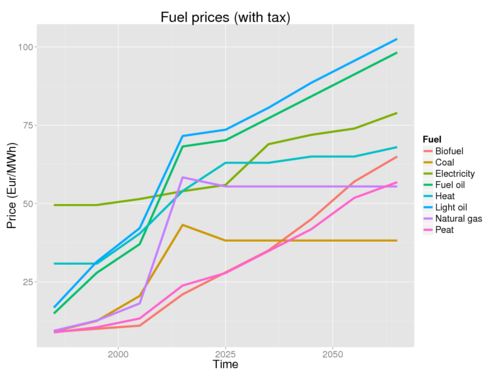
Prices of fuels in heat production without tax.
An example code for fetching and running the ovariable.
Rationale
This page contains prices for electricity, district heating, liquid fuels and consumer prices of hard coal, natural gas and domestic fuels in heat production in Finland. all data is based on knowledge of Statistics Finland In the end of data section there will be also data for maintenance and investment costs!!
This code calculates the price of fuels including tax.
Prices of fuels without tax
A previous version was based on several info sources [8]. However, this resulted in inconsistent prices between fuels. Now the table is simplified and made more robust using IEA estimates  VTT-R-03704-14_YDINPAP_(1) page 8, with the cost of accuracy. There should be an expert panel discussing the interdependencies of fuel prices to get the correct order.
Fuel prices(€ /MWh)| Obs | Fuel | 1985 | 1995 | 2005 | 2015 | 2025 | 2035 | 2045 | 2055 | 2065 | Description |
|---|
| 1 | Coal | 8.5 | 9.41 | 13.78 | 20 | 15 | 15 | 15 | 15 | 15 | |
| 2 | Gas | 9.1 | 11.6 | 16.2 | 42.9 | 40 | 40 | 40 | 40 | 40 | |
| 3 | Natural gas | 9.1 | 11.6 | 16.2 | 42.9 | 40 | 40 | 40 | 40 | 40 | Same as gas. |
| 4 | Oil | 14.3 | 25 | 32 | 52 | 54 | 61 | 68 | 75 | 82 | |
| 5 | Crude oil | 14.3 | 25 | 32 | 52 | 54 | 61 | 68 | 75 | 82 | Same as oil. |
| 6 | Fuel oil | 14.3 | 25 | 32 | 52 | 54 | 61 | 68 | 75 | 82 | Same as oil. |
| 7 | Heavy oil | 14.3 | 25 | 32 | 52 | 54 | 61 | 68 | 75 | 82 | Same as oil. |
| 8 | Light oil | 16 | 28 | 35 | 55 | 57 | 64 | 72 | 79 | 86 | Slightly higher than oil. |
| 9 | Bio | 9 | 10 | 11 | 21 | 28 | 35 | 45 | 57 | 76 | |
| 10 | Biofuel | 9 | 10 | 11 | 21 | 28 | 35 | 45 | 57 | 65 | Same as bio. |
| 11 | Peat | 6.6 | 8 | 9.8 | 17 | 21 | 28 | 35 | 45 | 50 | |
| 12 | Electricity | 40 | 40 | 40 | 40 | 42 | 55 | 58 | 60 | 65 | |
| 13 | Heat | 30.8 | 30.8 | 40.4 | 53.99 | 63 | 63 | 65 | 65 | 68 | |
| 14 | Cooling | 30.8 | 30.8 | 40.4 | 53.99 | 63 | 63 | 65 | 65 | 68 | Same as heat |
All prices are in 2015 euros.
Coal, Gas/Natural Gas, Light oil and Bio/Biofuel and Peat data from Statistics Finland[22]. Bio/Biofuel stands for wood chips.
Oil prices from U.S. Energy Information Administration[23]. All values converted first to 2015 dollars (inflation correction) and then to 2015 euros using the current (21.7.2015) exchange ratio of 1 $ = 0.923 €. Price per barrel then converted to price per MWh presuming that the energy released by burning one barrel is about 5.8 x 10⁶ BTU = 1.7 MWh, U.S. Internal Revenue Service[24].
Compound Annual Growth Rates (CAGR) for Coal, Gas/Natural Gas, Oil, Crude oil, Fuel oil, Heavy oil and Light oil from U.S. Energy Information Administration's "Annual Energy Outlook 2015 with projections to 2040" [25]. CAGR for Bio/Biofuel and Peat estimated to be 2 %, based on the price history.
Price of electricity [9].D↷
District heating data is based on the price for an apartment building (volume 10 000 m3, energy need 450 MWh/a). Data from Statistics Finland [10]. We assume that the price of district cooling is the same (although district cooling has been available only for a few years).
Uncertainties are assumed in the same way for all fuels: a certain percentage up and down from the best estimate, varying by year. The following uncertainties were used: 2025 5 %, 2035 10 %, 2045 15 %, 2055 20 %, 2065 30 %. It should be noted that uncertainties are different for different fuels, but we were unable to estimate fuel-specific uncertainties.
Taxes for different fuels
| Show details
|
Taxes of fuels(c€/l,c€/l,c€/l,c€/l,c€/kg,€/t,€/MWh,€/MWh,€/MWh,c€/kWh)| Obs | Time | Tax | Petrol | Diesel | Light fuel oil | Heavy fuel oil | Coal | Natural gas | Peat | Biofuel | Electricity | Description |
|---|
| 1 | 1.9.1990 | Product tax | 21.53 | 16.82 | 0.34 | 0.34 | 2.69 | 0.17 | 0.34 | 0 | | | | 2 | 1.1.1991 | Product tax | 26.57 | 17.49 | 0.35 | 0.35 | 2.83 | 0.18 | 0.35 | 0 | | | | 3 | 1.1.1992 | Product tax | 28.26 | 17.49 | 0.35 | 0.35 | 2.83 | 0.18 | 0.35 | 0 | | | | 4 | 1.8.1992 | Product tax | 31.62 | 17.49 | 0.35 | 0.35 | 2.83 | 0.18 | 0.35 | 0 | | | | 5 | 1.1.1993 | Product tax | 39.52 | 19.17 | 1.41 | 1.12 | 5.61 | 0.35 | 0.70 | 0 | 0.25 | | | 6 | 1.7.1993 | Product tax | 39.52 | 16.65 | 1.41 | 1.12 | 5.61 | 0.35 | 0.70 | 0 | 0.25 | | | 7 | 1.1.1994 | Product tax | 40.05 | 17.29 | 2.05 | 1.98 | 11.30 | 1.09 | 0.35 | 0 | | | | 8 | 1.1.1995 | Product tax | 45.12 | 27.50 | 3.02 | 3.12 | 19.53 | 0.94 | 0.59 | 0 | | | | 9 | 1.1.1996 | Product tax | 51.85 | 27.50 | 3.02 | 3.12 | 19.53 | 0.94 | 0.59 | 0 | | | | 10 | 1.1.1997 | Product tax | 51.85 | 27.50 | 4.88 | 3.72 | 28.42 | 1.19 | 0.71 | 0 | 0.40 | | | 11 | 1.4.1997 | Product tax | 51.85 | 27.50 | 4.88 | 3.72 | 28.42 | 1.19 | 0.71 | 0 | 0.24 | | | 12 | 1.1.1998 | Product tax | 55.22 | 30.02 | 5.50 | 4.34 | 33.40 | 1.40 | 0.82 | 0 | 0.34 | | | 13 | 1.9.1998 | Product tax | 55.22 | 30.02 | 6.37 | 5.40 | 41.37 | 1.73 | 1.51 | 0 | 0.42 | | | 14 | 1.1.2003 | Product tax | 58.08 | 31.59 | 6.71 | 5.68 | 43.52 | 1.82 | 1.59 | 0 | 0.44 | | | 15 | 1.7.2005 | Product tax | 58.08 | 31.59 | 6.71 | 5.68 | 43.52 | 1.82 | | 0 | 0.44 | | | 16 | 1.1.2007 | Product tax | 58.08 | 31.59 | 6.71 | 5.68 | 43.52 | 1.82 | | 0 | 0.22 | | | 17 | 1.1.2008 | Product tax | 62.02 | 36.05 | 8.35 | 6.42 | 49.32 | 2.016 | | 0 | 0.25 | | | 18 | 1.1.2011 | Product tax | 62.02 | 36.05 | 15.70 | 18.51 | 126.91 | 8.94 | 1.90 | 0 | 0.69 | | | 19 | 1.1.2012 | Product tax | 64.36 | 46.60 | 15.70 | 18.51 | 126.91 | 8.940 | 1.90 | 0 | 0.69 | | | 20 | 1.1.2013 | Product tax | 64.36 | 46.60 | 15.99 | 18.93 | 131.53 | 11.38 | 4.90 | 0 | 0.69 | | | 21 | 1.1.2014 | Product tax | 66.61 | 49.31 | 15.99 | 18.93 | 131.53 | 11.38 | 4.90 | 0 | 0.69 | | | 22 | 1.1.2015 | Product tax | 66.61 | 49.31 | 15.99 | 18.93 | 153.24 | 15.36 | 3.40 | 0 | 0.69 | | | 23 | 1.1.2011 | Energy content tax | 50.36 | | 7.70 | 8.79 | 54.54 | 3.00 | | 0 | | | | 24 | 1.1.2012 | Energy content tax | 50.36 | 30.70 | 7.70 | 8.79 | 54.54 | 3.00 | | 0 | | | | 25 | 1.1.2013 | Energy content tax | 50.36 | 30.70 | 6.65 | 7.59 | 47.10 | 4.45 | | 0 | | | | 26 | 1.1.2015 | Energy content tax | 50.36 | 30.70 | 6.65 | 7.59 | 47.10 | 6.65 | | 0 | | | | 27 | 1.1.2011 | Carbon dioxide tax | 11.66 | | 8.00 | 9.72 | 72.37 | 5.94 | | 0 | | | | 28 | 1.1.2012 | Carbon dioxide tax | 14.00 | 15.90 | 8.00 | 9.72 | 72.37 | 5.94 | | 0 | | | | 29 | 1.1.2013 | Carbon dioxide tax | 14.00 | 15.90 | 9.34 | 11.34 | 84.43 | 6.93 | | 0 | | | | 30 | 1.1.2014 | Carbon dioxide tax | 16.25 | 18.61 | 9.34 | 11.34 | 84.43 | 6.93 | | 0 | | | | 31 | 1.1.2015 | Carbon dioxide tax | 16.25 | 18.61 | 9.34 | 11.34 | 106.14 | 8.71 | | 0 | | | | 32 | 1.1.2011 | Energy tax | | | | | | | 1.90 | 0 | 0.69 | | | 33 | 1.1.2013 | Energy tax | | | | | | | 4.90 | 0 | 0.69 | | | 34 | 1.1.2014 | Energy tax | | | | | | | 4.90 | 0 | 0.69 | | | 35 | 1.1.2015 | Energy tax | | | | | | | 3.40 | 0 | 0.69 | | | 36 | 1.7.1984 | Maintenance and supply security fees | 0.72 | 0.39 | 0.39 | 0.32 | 1.48 | | | 0 | | | | 37 | 1.1.1997 | Maintenance and supply security fees | 0.68 | 0.35 | 0.35 | 0.28 | 1.18 | 0.084 | | 0 | 0.013 | | | 38 | 1.1.1990 | Oil pollution fees | 0.28 | 0.031 | 0.031 | 0.037 | | | | 0 | | | | 39 | 1.1.2005 | Oil pollution fees | 0.038 | 0.042 | 0.042 | 0.050 | | | | 0 | | | | 40 | 1.1.2010 | Oil pollution fees | 0.113 | 0.126 | 0.126 | 0.150 | | | | 0 | | |
|
Taxes and fees for fuel and energy production[26]
| Taxes and fees from |
Petrol (snt/l) |
Diesel (snt/l) |
Light fuel oil (snt/l) |
Heavy fuel oil (snt/kg) |
Coal (€/t) |
Natural gas (€/MWh) |
Peat (€/MWh)
|
| 1.1.1990 |
21,53 |
16,82 |
0,34 |
0,34 |
2,69 |
0,17 |
0,34
|
| 1.1.1991 |
26,57 |
17,49 |
0,35 |
0,35 |
2,83 |
0,18 |
0,35
|
| 1.1.1992 |
28,26 |
17,49 |
0,35 |
0,35 |
2,83 |
0,18 |
0,35
|
| 1.8.1992 |
31,62 |
17,49 |
0,35 |
0,35 |
2,83 |
0,18 |
0,35
|
| 1.1.1993 |
39,52 |
19,17 |
1,41 |
1,12 |
5,61 |
0,35 |
0,70
|
| 1.7.1993 |
39,52 |
16,65 |
1,41 |
1,12 |
5,61 |
0,35 |
0,70
|
| 1.1.1994 |
40,05 |
17,29 |
2,05 |
1,98 |
11,30 |
1,09 |
0,35
|
| 1.1.1995 |
45,12 |
27,50 |
3,02 |
3,12 |
19,53 |
0,94 |
0,59
|
| 1.1.1996 |
51,85 |
27,50 |
3,02 |
3,12 |
19,53 |
0,94 |
0,59
|
| 1.1.1997 |
51,85 |
27,50 |
4,88 |
3,72 |
28,42 |
1,19 |
0,71
|
| 1.4.1997 |
51,85 |
27,50 |
4,88 |
3,72 |
28,42 |
1,19 |
0,71
|
| 1.1.1998 |
55,22 |
30,02 |
5,50 |
4,34 |
33,40 |
1,40 |
0,82
|
| 1.9.1998 |
55,22 |
30,02 |
6,37 |
5,40 |
41,37 |
1,73 |
1,51
|
| 1.1.2003 |
58,08 |
31,59 |
6,71 |
5,68 |
43,52 |
1,82 |
1,59
|
| 1.7.2005 |
58,08 |
31,59 |
6,71 |
5,68 |
43,52 |
1,82 |
-
|
| 1.1.2007 |
58,08 |
31,59 |
6,71 |
5,68 |
43,52 |
1,82 |
-
|
| 1.1.2008 |
62,02 |
36,05 |
8,35 |
6,42 |
49,32 |
2,016 |
-
|
| 1.1.2011 |
62,02 |
36,05 |
15,70 |
18,51 |
126,91 |
8,94 |
1,90
|
| 1.1.2012 |
64,36 |
46,60 |
15,70 |
18,51 |
126,91 |
8,940 |
1,90
|
| 1.1.2013 |
64,36 |
46,60 |
15,99 |
18,93 |
131,53 |
11,38 |
4,90
|
| 1.1.2014 |
66,61 |
49,31 |
15,99 |
18,93 |
131,53 |
11,38 |
4,90
|
| 1.1.2015 |
66,61 |
49,31 |
15,99 |
18,93 |
153,24 |
15,36 |
3,40
|
| Energy content tax
|
| 1.1.2011 |
50,36 |
- |
7,70 |
8,79 |
54,54 |
3,00 |
-
|
| 1.1.2012 |
50,36 |
30,70 |
7,70 |
8,79 |
54,54 |
3,00 |
-
|
| 1.1.2013 |
50,36 |
30,70 |
6,65 |
7,59 |
47,10 |
4,45 |
-
|
| 1.1.2015 |
50,36 |
30,70 |
6,65 |
7,59 |
47,10 |
6,65 |
-
|
| Carbondioxide tax
|
| 1.1.2011 |
11,66 |
- |
8,00 |
9,72 |
72,37 |
5,94 |
-
|
| 1.1.2012 |
14,00 |
15,90 |
8,00 |
9,72 |
72,37 |
5,94 |
-
|
| 1.1.2013 |
14,00 |
15,90 |
9,34 |
11,34 |
84,43 |
6,93 |
-
|
| 1.1.2014 |
16,25 |
18,61 |
9,34 |
11,34 |
84,43 |
6,93 |
-
|
| 1.1.2015 |
16,25 |
18,61 |
9,34 |
11,34 |
106,14 |
8,71 |
-
|
| Energy tax
|
| 1.1.2011 |
- |
- |
- |
- |
- |
- |
1,90
|
| 1.1.2013 |
- |
- |
- |
- |
- |
- |
4,90
|
| 1.1.2014 |
- |
- |
- |
- |
- |
- |
4,90
|
| 1.1.2015 |
- |
- |
- |
- |
- |
- |
3,40
|
| Maintenance and supply sercurity fees
|
| 1.7.1984 |
0,72 |
0,39 |
0,39 |
0,32 |
1,48 |
- |
-
|
| 1.1.1997 |
0,68 |
0,35 |
0,35 |
0,28 |
1,18 |
0,084 |
-
|
| Oil pollution fees
|
| 1.1.1990 |
0,28 |
0,031 |
0,031 |
0,037 |
- |
- |
-
|
| 1.1.2005 |
0,038 |
0,042 |
0,042 |
0,050 |
- |
- |
-
|
| 1.1.2010 |
0,113 |
0,126 |
0,126 |
0,150 |
- |
- |
-
|
+ Show code- Hide code
library(OpasnetUtils)

fuelTaxRaw <- Ovariable("fuelTaxRaw", ddata = "Op_en4151.taxes_of_fuels")

fuelTax <- Ovariable(
	"fuelTax",
	dependencies = data.frame(Name = "fuelTaxRaw"),#, Ident = "Op_en4151/fuelTaxRaw"),
	formula = function(...) {
		#taxes <- fuelTaxRaw
		#taxes$Result <- as.numeric(as.character(taxes$Result))

		#units <- c("c€/l","c€/l","c€/l","c€/kg","€/t","€/MWh","c€/kWh")
		#taxes$Units <- units

		# convert units into €/MWh
		# energy densities/specific energies from
		# http://webserver.dmt.upm.es/~isidoro/bk3/c15/Fuel%20properties.pdf
		# and https://en.wikipedia.org/wiki/Energy_density
		conversion <- c(
				1/32.4*60*60/100,
				1/35.8*60*60/100,
				1/35.8*60*60/100,
				1/43*60*60/100,
				1/24/1000*60*60,
				1,
				1,
				1,
				10
		)
		fuels <- c("Petrol", "Diesel", "Light fuel oil", "Heavy fuel oil", "Coal", "Natural gas", "Peat", "Biofuel", "Electricity")
		conversion <- Ovariable(
			output = data.frame(
				Fuel = fuels,
				Result = conversion
			)
		)
		#taxes$Result <- taxes$Result * conversion
		taxes <- fuelTaxRaw * conversion

		alias <- Ovariable(output = data.frame(
			Fuel = rep(fuels, c(0,0,1,4,0,2,0,2,0)),
			Fuel2 = c("Light oil", "Oil", "Crude oil", "Fuel oil", "Heavy oil", "Natural gas", "Gas", "Biofuel", "Bio")
		))
		taxes <- merge(taxes, alias, all.x = TRUE)
		temp <- as.character(taxes$Fuel2)
		temp[is.na(temp)] <- as.character(taxes$Fuel[is.na(temp)])
		taxes$Fuel <- temp
		taxes$Fuel2 <- NULL

		taxes <- taxes[!is.na(result(taxes)),]
		taxes <- taxes[!taxes$Tax %in% c("Energy content tax", "Carbon dioxide tax"),]
		#taxes <- oapply(taxes, NULL, sum, "Tax")
		taxes$Time  <- as.POSIXct(strptime(as.character(taxes$Time), format = "%d.%m.%Y"))

		return(taxes)
	}
)

objects.store(fuelTaxRaw, fuelTax)
| |
Energy balance
Question
What is energy balance and how is it modelled?
Answer
Summing up the amount of energy produced and subtracting the amount of energy consumed within a time period gives the energy balance. Since the electricity grid and district heat network lack significant storage mechanics, the balance has to be virtually zero over short periods. When considering the balance of a particular area (e.g. Helsinki), we can make the assumption that electricity can be imported and exported in international markets. The energy in the district heat network, however, has to be produced locally. This sets up the non-trivial problem of optimising production so that there are no significant deficits as well as minimising losses and maximising profits. This problem is solved (to some extent) by market forces in the real world.
In Opasnet, there are two different ways to calculate energy balance. Our most recent energy balance model uses linear programming tools to solve an optimum for the activity of a given set of production units in simulated instances created by the main model. The main model is responsible for the decision making aspects, while the energy balance optimisation only functions as an approximation of real world market mechanics. This version was used in Helsinki energy decision 2015.
The previous version was based on setting up a set of linear equations describing the inputs, outputs, and shares of different energy and plant processes. This approach is less flexible, because it does not use an optimising function and everything must be described as linear (or piecewise linear). However, this approach was successfully used in Energy balance in Kuopio and Energy balance in Suzhou.
Example of energy balance model: Incomes and costs of energy production in Helsinki. The scenarios are from the assessment Helsinki energy decision 2015.
This code is an example how the energy balance model is used in a city case. The data comes from Helsinki energy decision 2015.
Rationale
Energy balance with linear programming
The linear programming problem is set up as follows.
For each production unit: let xi be activity of the plant. Lets also have variables yj for deficits and excesses for each type of energy produced.
The objective function is the function we are optimising. Each production unit has a unit profit per activity denoted by ai which is determined by the amount of different input commodities (e.g. coal) per amount of different output commodities (i.e. electricity and heat) and their market prices. Also, lets say we want to make sure that district heat demand is always met when possible and have a large penalty factor for each unit of heat demand not met (1 M€ in the model). In addition, it must be noted that excess district heat becomes wasted so it counts as loss. Let these deficit and excess related losses be denoted by bj. The whole objective function then becomes: sum(xiai) + sum(yjbj).
The values of variables are constrained by equalities and inequalities: the sum of production of a commodity is equal to its demand minus deficit plus excess, activity is constrained by the maximum capacity and all variables are non-negative by definition.
This can be efficiently solved by computers for each given instance. Production wind-up and wind-down is ignored, since time continuity is not considered. As a consequence fuel limits (e.g. diminishing hydropower capacity) are not modelled completely either.
- Ovariables like EnergyNetworkOptim below are used in Helsinki energy decision 2015. Prices of fuels in heat production are used as direct inputs in the optimising.
+ Show code- Hide code
## This code is  Op_en5141/EnergyNetworkOptim [[Energy balance]].
library(OpasnetUtils)

EnergyConsumerDemandTotal <- Ovariable("EnergyConsumerDemandTotal",
	dependencies = data.frame(
		Name = c(
			"EnergyConsumerDemand"
		)
	),
	formula = function(...) {
		energy <- oapply(EnergyConsumerDemand, NULL, sum, c("Renovation", "Efficiency"))
		energy <- energy * 1e-6 # W to MW
		return(energy)
	}
)

EnergyFlowHeat <- Ovariable("EnergyFlowHeat",
	dependencies = data.frame(
		Name = c(
			"EnergyConsumerDemandTotal",
			"fuelShares"
		)
	),
	formula = function(...) {
		EnergyFlowHeat <- EnergyConsumerDemandTotal[EnergyConsumerDemandTotal$Consumable %in% c("Heating", "Hot water"),] * fuelShares
		return(EnergyFlowHeat)
	}
)

EnergyFlowOther <- Ovariable("EnergyFlowOther",
	dependencies = data.frame(
		Name = c(
			"EnergyConsumerDemandTotal",
			"temperene",
			"nontemperene"
		)
	),
	formula = function(...) {
		EnergyFlowOther <- merge(
				EnergyConsumerDemandTotal[!EnergyConsumerDemandTotal$Consumable %in% c("Heating", "Hot water"),],
				unique(OpasnetUtils::combine(temperene, nontemperene)[,c("Consumable", "Fuel")])
		)
		EnergyFlowOther@name <- EnergyConsumerDemandTotal@name
		return(EnergyFlowOther)
	}
)

EnergyNetworkDemand <- Ovariable("EnergyNetworkDemand",
	dependencies = data.frame(
		Name = c(
			"EnergyFlowHeat",
			"EnergyFlowOther",
			"EnergyConsumerDemandTotal"
		)
	),
	formula = function(...) {
		demand <- OpasnetUtils::combine(
				EnergyFlowHeat[EnergyFlowHeat$Fuel %in% c("Heat", "Electricity"), colnames(EnergyFlowHeat@output) != "Burner"],
				EnergyFlowOther[EnergyFlowOther$Fuel %in% c("Cooling", "Electricity"),]
		)

		# EnergyFlowOther should not have other flows
		#assign("EnergyFlowOther", NULL, .GlobalEnv)

		#assign("EnergyFlowHeat", EnergyFlowHeat[!EnergyFlowHeat$Fuel %in% c("Heat", "Electricity"),], .GlobalEnv)

		# Total consumer demand also unnecessary?
		#assign("EnergyConsumerDemandTotal", NULL, .GlobalEnv)

		NAindex <- sapply(lapply(lapply(demand@output, unique), is.na), sum)
		NAindex <- names(NAindex)[NAindex != 0]

		demand@output <- fillna(demand@output , NAindex)
		demand <- oapply(demand, NULL, sum, c("Heating", "Consumable"))#, "Renovation", "Efficiency")) # Assumes no NA

		return(demand)
	}
)

EnergyNetworkOptim <- Ovariable("EnergyNetworkOptim",
	dependencies = data.frame(
		Name = c(
			#"energy", # Energy supply and demand in the system
			#"nondynsupply", # Energy supply that is not optimised.
			#"requiredName", # Fuel name for the energy type that is balanced for inputs and outputs.
			#"fuelShares", # Shares of fuels for different heating types.
			"energyProcess", # Matrix showing inputs and outputs of the process of each plant.
			"fuelPrice", # Prices of fuels (by Time)
			#"timelylimit", # Maximum energy supply in the given conditions at a particular time point
			"plantParameters", # Capacities and costs of running each plant
			#"temperene",
			#"nontemperene",
			"EnergyNetworkDemand"
		),
		Ident = c(
			#NA,
			#NA,
			#NA,
			#NA,
			NA,
			"Op_en4151/fuelPrice",
			#NA,
			NA,
			#"Op_en5488/temperene",
			#"Op_en5488/nontemperene",
			NA
		)
	),
	formula = function(...) {

		require(lpSolve)
		require(plyr)
		require(reshape2)

		# Prices are given as €/MWh while plant activity is given as MW while optimisation is done
		# with time resolution = 1 day
		optim_time_period_adj <- 24

		# List non-interating indices

		exclude <- c("Fuel", "Plant", "Parameter", "Heating", "Consumable", "Burner")

		# Calculate unitprofit for plant activity energy flows

		unitp <- fuelPrice * energyProcess * optim_time_period_adj
		unitp <- oapply(unitp, NULL, sum, c("Fuel", "Burner"))
		colnames(unitp@output)[colnames(unitp@output) == "Result"] <- "UnitPrice"

		# Reshape crucial variables to reduce merging difficulty

		ePmargs <- colnames(energyProcess@output)[energyProcess@marginal]
		energyProcess@output <- dcast(
			energyProcess@output,
			as.formula(paste(paste(ePmargs[ePmargs != "Fuel"], collapse = "+"), "~ Fuel")),
			value.var = paste(energyProcess@name, "Result", sep = ""),
			fill = NA
		)
		energyProcess@marginal <- colnames(energyProcess@output) %in% ePmargs

		pPmargs <- colnames(plantParameters@output)[plantParameters@marginal]
		plantParameters@output <- dcast(
				plantParameters@output,
				as.formula(paste(paste(pPmargs[pPmargs != "Parameter"], collapse = "+"), "~ Parameter")),
				value.var = paste(plantParameters@name, "Result", sep = ""),
				fill = NA
		)
		plantParameters@marginal <- colnames(plantParameters@output) %in% pPmargs

		EnergyNetworkDemand$Fuel <- paste(EnergyNetworkDemand$Fuel, "Demand", sep = "")
		ENDmargs <- colnames(EnergyNetworkDemand@output)[EnergyNetworkDemand@marginal]
		EnergyNetworkDemand@output <- dcast(
				EnergyNetworkDemand@output,
				as.formula(paste(paste(ENDmargs[ENDmargs != "Fuel"], collapse = "+"), "~ Fuel")),
				value.var = paste(EnergyNetworkDemand@name, "Result", sep = ""),
				fill = NA
		)
		EnergyNetworkDemand@marginal <- colnames(EnergyNetworkDemand@output) %in% ENDmargs

		fuelPrice$Fuel <- paste(fuelPrice$Fuel, "Price", sep = "")
		fPmargs <- colnames(fuelPrice@output)[fuelPrice@marginal]
		fuelPrice@output <- dcast(
				fuelPrice@output,
				as.formula(paste(paste(fPmargs[fPmargs != "Fuel"], collapse = "+"), "~ Fuel")),
				value.var = paste(fuelPrice@name, "Result", sep = ""),
				fill = 0
		)
		fuelPrice@marginal <- colnames(fuelPrice@output) %in% fPmargs

		# Duplicates a couple of values, but provides better performance
		vars <- merge(EnergyNetworkDemand, plantParameters)
		vars <- merge(vars, energyProcess)
		vars <- merge(vars, fuelPrice)
		vars <- merge(vars, unitp)

		# Split into iterations
		#vars <- dlply(vars@output, colnames(vars@output)[vars@marginal & !colnames(vars@output) %in% exclude], I)

		#out <- data.frame()

		include <- union(ePmargs, pPmargs)
		include <- union(include, ENDmargs)
		include <- union(include, fPmargs)
		include <- include[!include %in% exclude]

		# Optimisation iteration function

		optf <- function(varsi) {

			# Acquire relevant sections of variables with respect to index iteration

			demandi <- unlist(varsi[1,grepl("Demand$", colnames(varsi))])
			names(demandi) <- gsub("Demand$", "", names(demandi))

			fuelPricei <- unlist(varsi[1,grepl("Price$", colnames(varsi))])
			names(fuelPricei) <- gsub("Price$", "", names(fuelPricei))
			fuelPricei <- fuelPricei[names(fuelPricei) != "Unit"]

			plants <- as.character(unique(varsi[["Plant"]])) # Used for ordering parameters
			if (nrow(varsi) != length(plants)) stop("Wrong subset given to energy production optimizer! Each row not unique with respect to Plant.")

			lower <- varsi[["Min"]]

			upper <- varsi[["Max"]]

			opcost <- varsi[["Operation cost"]]

			unitpi <- varsi[["UnitPrice"]]

			#commodities <- as.character(unique(energyProcessi$Fuel)) # Used for ordering parameters

			# Constraint matrix

			# Total number of variables:
			# * plant activity for each plant
			# * (commodity flow total)
			# * commodity deficit and excess with respect to demand
			# * opeartion costs
			nvars <- length(plants) + length(demandi) * 2 + 1

			# Rows:
			# * demand rows and their constraints
			# * (commodity flow rows)
			# * plant activity constraints
			# * operation costs row
			nrows <- 3 * length(demandi) + 2 * length(plants) + 1
			M <- matrix(
				0,
				nrows,
				nvars
			)

			sign <- rep(">=", nrows)
			constant <- rep(0, nrows)

			for (j in 1:length(demandi)) {
				# Total flow (production - consumption between all processes) + deficit = demand + excess
				# which translates to:
				# total_commodity_flow + deficit - excess == constant ("static" demand)

				M[j, length(plants) + j*2 + 1:2 - 2] <- c(1, -1)
				sign[j] <- "=="
				constant[j] <- demandi[j]

				# Plant flows by activity
				M[j, 1:length(plants)] <- varsi[[names(demandi)[j]]]

			}

			rowi <- length(demandi)
			diag(M[
				(rowi + 1):(rowi + length(plants)),
				1:length(plants)
			]) <- 1
			diag(M[
				(rowi + length(plants) + 1):(rowi + 2 * length(plants)),
				1:length(plants)
			]) <- 1
			constant[rowi + 1:length(plants)] <- lower
			constant[rowi + length(plants) + 1:length(plants)] <- upper
			sign[rowi + length(plants) + 1:length(plants)] <- "<="

			rowi <- rowi + 2 * length(plants)
			# Excess and deficit must both be positive
			diag(M[
				rowi + 1:(2 * length(demandi)),
				length(plants) + #length(commodities) +
						1:(2 * length(demandi))
			]) <- 1

			# Operating cost
			M[nrows, 1:length(plants)] <- opcost * optim_time_period_adj
			M[nrows, nvars] <- -1
			sign[nrows] <- "=="

			# Objective function (profits - penalty)
			objective <- rep(0, nvars)
			# Commodity prices
			#objective[length(plants) + (1:length(commodities))[!is.na(fuelPricej)]] <- result(fuelPricei)[fuelPricej[!is.na(fuelPricej)]]
			# Penalize heat deficit heavily,
			# electricity deficit has no impact on profit assuming company sells to customers at the purchase price
			# cooling deficit has no effect
			if ("Heat" %in% names(demandi)) {
				objective[length(plants) + match("Heat", names(demandi)) * 2 - 1] <- -1e6
			}

			# Electricity excess can be sold in the markets,
			# heat and cooling (and other?) excess, however, cannot, hence they need to be deducted from profits
			objective[
				length(plants) + which(names(demandi) != "Electricity") * 2
			] <- - fuelPricei[match(names(demandi)[names(demandi) != "Electricity"], names(fuelPricei))] * optim_time_period_adj

			# Operation cost
			objective[nvars] <- -1

			# Unit profit
			objective[1:length(plants)] <- unitpi

			# Do actual linear programming
			temp <- lp(
				"max",
				objective,
				M,
				sign,
				constant
			)

			# Format results
			outi <- varsi[rep(1, nvars + 1), include, drop = FALSE]
			outi[["Process_variable_type"]] <- rep(
				c("Activity", "Flow", "Misc"),
				c(length(plants), nvars - length(plants) - 1, 2)
			)
			outi[["Process_variable_name"]] <- c(
				as.character(plants),
				paste(rep(names(demandi), each = 2), c("Deficit", "Excess"), sep = ""),
				"Operation cost",
				"Profit"
			)
			outi[["Result"]] <- c(temp$solution, temp$objval)

			return(outi)
		}
		#aggregate(out$Result[out$Process_variable_name == "Profit"], out[out$Process_variable_name == "Profit",colnames(out) %in% c("Time", "Temperature") | grepl("Policy", colnames(out))], mean)
		#aggregate(out$Result[out$Process_variable_name == "HeatDeficit"], out[out$Process_variable_name == "HeatDeficit", colnames(out) %in% c("Time", "Temperature") | grepl("Policy", colnames(out))], mean)
		#aggregate(out$Result[out$Process_variable_name == "Hanasaari"], out[out$Process_variable_name == "Hanasaari", colnames(out) %in% c("Time", "Temperature") | grepl("Policy", colnames(out))], mean)

		# Error handling
		optfsecure <- function(varsi) {
			ret <- tryCatch(
				optf(varsi),
				error = function(e) return(NULL)
			)
			if (!is.null(ret)) {
				return(ret)
			} else {
				warning(paste("EnergyNetworkOptim failed optimising a permutation with error:", geterrmessage()))
				return(data.frame())
			}
		}

		out <- ddply(vars@output, colnames(vars@output)[vars@marginal & !colnames(vars@output) %in% exclude], optfsecure)

		out <- Ovariable(output = out, marginal = !grepl("Result$", colnames(out)))

		return(out)
	}
)

fuelUse <- Ovariable("fuelUse",
	dependencies = data.frame(
		Name = c(
			"EnergyNetworkOptim",
			"EnergyNetworkDemand",
			"energyProcess",
			"EnergyFlowHeat",
			"temperdays"
		)
	),
	formula = function(...){

		# Calculate flows resulting from plant activity
		EnergyFlow <- EnergyNetworkOptim[EnergyNetworkOptim$Process_variable_type == "Activity", colnames(EnergyNetworkOptim@output) != "Process_variable_type"]
		colnames(EnergyFlow@output)[colnames(EnergyFlow@output) == "Process_variable_name"] <- "Plant"

		EnergyFlow <- EnergyFlow * energyProcess

		# Realised consumption of centrally produced commodities (demand - deficit or prod - excess)
		# NOTE: centralized flows which consume electricity for example should be separated
		# from consumer demand and consumption, so prod - excess is not accurate
		deficit <- EnergyNetworkOptim[
				grepl("Deficit$", EnergyNetworkOptim$Process_variable_name),
				colnames(EnergyNetworkOptim@output) != "Process_variable_type"
		]
		colnames(deficit@output)[colnames(deficit@output) == "Process_variable_name"] <- "Fuel"
		deficit$Fuel <- gsub("Deficit$", "", deficit$Fuel)
		# Assume that the power company purchases any electricity deficit from the markets in order to satisfy demand
		result(deficit)[deficit$Fuel == "Electricity"] <- 0

		#excess <- EnergyNetworkOptim[
		#		grepl("Excess$", EnergyNetworkOptim$Process_variable_name),
		#		colnames(EnergyNetworkOptim@output) != "Process_variable_type"
		#]
		#colnames(excess@output)[colnames(excess@output) == "Process_variable_name"] <- "Fuel"
		#excess$Fuel <- gsub("Excess$", "", excess$Fuel)

		#temp <- oapply(EnergyFlow, NULL, sum, c("Plant", "Burner"))

		#real <- oapply(EnergyFlow[EnergyFlow$Fuel %in% unique(excess$Fuel)], NULL, sum, c("Plant", "Burner"))
		#real <- real - excess

		real <- EnergyNetworkDemand - deficit

		# Combine
		real$Burner <- "None"
		real$Plant <- "Domestic"

		heating <- EnergyFlowHeat[!EnergyFlowHeat$Fuel %in% unique(deficit$Fuel),]
		heating <- oapply(heating, NULL, sum, "Consumable")
		heating$Plant <- "Domestic"
		heating$Heating <- NULL

		EnergyFlow <- OpasnetUtils::combine(0 - EnergyFlow, real, heating)
		EnergyFlow <- unkeep(EnergyFlow, sources = TRUE, prevresults = TRUE)
		#EnergyFlowTest <- oapply(EnergyFlow, c("Time", "Temperature", "Fuel"), sum)
		#ggplot(EnergyFlowTest@output, aes(x = Temperature, y = Result, group = Fuel, color = Fuel)) + geom_line() + facet_wrap( ~ Time)

		EnergyFlow <- EnergyFlow * temperdays * 3600 * 24
		EnergyFlow <- oapply(EnergyFlow, cols = c("Temperature"), FUN = sum)
		return(EnergyFlow)
	}
)

EnergyNetworkCost <- Ovariable("EnergyNetworkCost",
	dependencies =
		data.frame(
			Name = c(
				"plantParameters",
				"EnergyNetworkOptim",
				"temperdays"
			),
			Ident = c(
				NA,
				"Op_en5141/EnergyNetworkOptim", # [[Energy balance]]
				NA
			)
		),
	formula = function(...) {

		oper <- plantParameters[plantParameters@output$Parameter == "Max" , colnames(plantParameters@output) != "Parameter"]
		result(oper)[result(oper) != 0] <- 1

		oper <- plantParameters * oper

		# Take the first year when a plant is operated and put all investment cost there.
		investment <- oper[oper@output$Parameter == "Investment cost" , colnames(oper@output) != "Parameter"]
		investment <- investment[result(investment) > 0 , ]
		investment <- investment[order(investment@output$Time) , ]
		investment <- investment[!duplicated(investment@output[investment@marginal & colnames(investment@output) != "Time"]) , ]
		investment <- unkeep(investment, sources = TRUE)
		#investment <- oapply(investment, cols = "Plant", FUN = sum)

		maintenance <- oper[oper@output$Parameter == "Management cost" , colnames(oper@output) != "Parameter"]
		maintenance <- unkeep(maintenance, sources = TRUE)
		#maintenance <- oapply(maintenance, cols = c("Plant"), FUN = sum)

		operation <- EnergyNetworkOptim[EnergyNetworkOptim@output$Process_variable_name == "Operation cost" , ]
		operation <- operation * temperdays * 10 * 1E-6 # For 10-year periods, € -> M€
		operation <- oapply(operation, cols = c("Temperature"), FUN = sum)
		operation <- unkeep(operation, cols = c("Process_variable_name", "Process_variable_type"), sources = TRUE, prevresults = TRUE)
		operation <- operation * Ovariable(output = data.frame(Plant = "Operation", Result = 1), marginal = c(TRUE, FALSE))
		cost <- OpasnetUtils::combine(investment, maintenance, operation)
		marginals <- character()
		for(i in colnames(cost@output)[cost@marginal]) {
			if(any(is.na(cost@output[[i]]))) marginals <- c(marginals, i)
		}
		if(length(marginals) > 0) {
			cost@output <- fillna(cost@output, marginals)
			warning(paste("In combine had to fillna marginals", marginals, "\n"))
		}

		return(cost)
	}
)

objects.store(EnergyConsumerDemandTotal, EnergyFlowHeat, EnergyFlowOther, EnergyNetworkDemand, EnergyNetworkOptim, fuelUse, EnergyNetworkCost)
cat("Ovariables EnergyConsumerDemandTotal, EnergyFlowHeat, EnergyFlowOther, EnergyNetworkDemand, EnergyNetworkOptim, EnergyNetworkCost and fuelUse stored.\n")
| |
Fuel use and fuel shares in generic processes
There is an alternative way for calculating fuel use. It is based on the idea that for each heating type, there is a constant share of fuels used. For some heating types, this is generic and is shown on this page. For some others, the constant is case-specific and is determined on a case-specific page.
The table below contains connections of heating types and fuel usage in generic situations. There may be case-specific differences, which must be handled separately.
Fuel use in different heating types(-)| Obs | Heating | Burner | Fuel | Fraction | Description |
|---|
| 1 | Wood | Household | Wood | 1 | |
| 2 | Oil | Household | Light oil | 1 | |
| 3 | Gas | Household | Gas | 1 | |
| 4 | Heating oil | Household | Light oil | 1 | |
| 5 | Coal | Household | Coal | 1 | |
| 6 | Other sources | Household | Other sources | 1 | |
| 7 | No energy source | Household | Other sources | 1 | |
| 8 | Geothermal | Grid | Electricity | 0.3 | Geothermal does not sum up to 1 because more heat is produced than electricity consumed. |
| 9 | Centrifuge, hydro-extractor | Grid | Electricity | 0.3 | Not quite clear what this is but presumably a heat pump. |
| 10 | Solar heater/ collector | Grid | Electricity | 0.1 | Use only; life-cycle impacts omitted. |
| 11 | Electricity | Grid | Electricity | 1 | |
| 12 | District | Undefined | Heat | 1 | |
Emission factors for burning processes
Question
What are the emission factors for burning processes and how to estimate emissions based on them? The focus is on the situation in Finland.
Answer
An example code for downloading and using the variable.
Rationale
HSY emission factors
This section describes the use of HSY emission factors used for CO2 emission estimates. This should be merged with the other data, but it is first described as such.
These emission factors are derived from the Helsinki Region Environmental Services (HSY) climate data [11] on 27th Nov 2018. Emission factors were initially calculated for every entry in the data file (4180 rows in total). Then, emission sectors were compared along timeline for each city separately. We noticed that several sectors shared practically the same emission factors with few differences, which are not plausible as real differences (Table Sector classification). So, we took a mean of the values to represent all sectors in the same EFclass group.
Then, we compared results from different cities. There were minor changes that may be due to some real differences in data, and also a some changes that looked like artefact. However, there were two sectors, namely district heating and fuels that clearly differed between cities in a plausible way. Therefore, we used city-specific emission factors for these two sectors and those of Helsinki for all other sectors (because Helsinki seemed to have the least amount of artefact in the data).
Sector classification(-)| Obs | Sector | Sektori | EFclass | PKluokka | dummy |
|---|
| 1 | metro | metrot | electricity | sähkö | 1 |
| 2 | trams | raitiovaunut | electricity | sähkö | 1 |
| 3 | local trains | lähijunat | electricity | sähkö | 1 |
| 4 | consumer electricity | kulutussähkö | electricity | sähkö | 1 |
| 5 | passenger ships | matkustajalaivat | ships | laivat | 1 |
| 6 | cargo ships | rahtilaivat | ships | laivat | 1 |
| 7 | buses | linja-autot | diesel machines | dieselkoneet | 1 |
| 8 | vans | pakettiautot | diesel machines | dieselkoneet | 1 |
| 9 | machinery | työkoneet | diesel machines | dieselkoneet | 1 |
| 10 | trucks | kuorma-autot | diesel machines | dieselkoneet | 1 |
| 11 | leasure boats | huviveneet | boats | veneet | 1 |
| 12 | professional boats | ammattiveneet | boats | veneet | 1 |
| 13 | district heating | kaukolämpö | district heating | kaukolämpö | 1 |
| 14 | oil heating | öljylämmitys | oil heating | öljylämmitys | 1 |
| 15 | electric heating | sähkölämmitys | electric heating | sähkölämmitys | 1 |
| 16 | geothermal heating | maalämpö | geothermal heating | maalämpö | 1 |
| 17 | fuels | polttoaineet | fuels | polttoaineet | 1 |
| 18 | processes | prosessit | processes | prosessit | 1 |
| 19 | private cars | henkilöautot | private cars | henkilöautot | 1 |
| 20 | motor cycles | moottoripyörät | motor cycles | moottoripyörät | 1 |
Sector hierarchy(-)| Obs | Class | Subclass | Luokka | Alaluokka | dummy |
|---|
| 1 | heating | district heating | lämmitys | kaukolämpö | 1 |
| 2 | heating | oil heating | lämmitys | öljylämmitys | 1 |
| 3 | heating | electric heating | lämmitys | sähkölämmitys | 1 |
| 4 | heating | geothermal heating | lämmitys | maalämpö | 1 |
| 5 | electricity | consumer electricity | sähkö | kulutussähkö | 1 |
| 6 | transport | road transport | liikenne | tieliikenne | 1 |
| 7 | transport | rail transport | liikenne | raideliikenne | 1 |
| 8 | transport | shipping | liikenne | laivaliikenne | 1 |
| 9 | industry and machinery | machinery | teollisuus ja työkoneet | työkoneet | 1 |
| 10 | industry and machinary | fuels | teollisuus ja työkoneet | polttoaineet | 1 |
| 11 | industry and machinery | processes | teollisuus ja työkoneet | prosessit | 1 |
| 12 | waste management | landfill | jätteiden käsittely | kaatopaikka | 1 |
| 13 | waste management | biowaste composting | jätteiden käsittely | biojätteen kompostointi | 1 |
| 14 | waste management | waste water treatment | jätteiden käsittely | jäteveden käsittely | 1 |
| 15 | waste management | waste water sludge composting | jätteiden käsittely | jätevesilietteen kompostointi | 1 |
| 16 | agriculture | fields | maatalous | pellot | 1 |
| 17 | agriculture | farm animals | maatalous | kotieläimet | 1 |
| 18 | road transport | private cars | tieliikenne | henkilöautot | 1 |
| 19 | road transport | motor cycles | tieliikenne | moottoripyörät | 1 |
| 20 | road transport | vans | tieliikenne | pakettiautot | 1 |
| 21 | road transport | trucks | tieliikenne | kuorma-autot | 1 |
| 22 | road transport | buses | tieliikenne | linja-autot | 1 |
| 23 | rail transport | local trains | raideliikenne | lähijunat | 1 |
| 24 | rail transport | metro | raideliikenne | metrot | 1 |
| 25 | rail transport | trams | raideliikenne | raitiovaunut | 1 |
| 26 | shipping | leasure boats | laivaliikenne | huviveneet | 1 |
| 27 | shipping | professional boats | laivaliikenne | ammattiveneet | 1 |
| 28 | shipping | passenger ships | laivaliikenne | matkustajalaivat | 1 |
| 29 | shipping | cargo ships | laivaliikenne | rahtilaivat | 1 |
Emission factors in Helsinki(ton/GWh)| Obs | Sector | 2015 | 2030 | 2035 |
|---|
| 1 | Consumer electricity | 121.5 | 70.6 | 45 |
| 2 | Electric heating | 234.2 | 138.5 | 88.3 |
| 3 | District heating | 189.7 | 128.8 | 49.1 |
| 4 | Natural gas | 198 | 198 | 198 |
| 5 | Light fuel oil | 261 | 261 | 261 |
| 6 | Coal | 341 | 341 | 341 |
The data above comes from Gaia report [12].
Inputs and calculations
Variables needed for calculating emissions.
| Dependencies |
Measure |
Indices |
Missing data
|
| fuelUse (from Energy balance or other relevant source)
|
Amount of fuel used per timepoint.
|
Required indices: Fuel. Typical indices: Plant
|
|
| emissionsLocations (case-specific knowledge from e.g. Helsinki energy production)
|
Tells how where emissions occur and from how high a stack.
|
Required indices: - . Typical indices: Plant
|
|
| emissionFactors (generic information, but may be cultural differences. E.g. Emission factors for burning processes ##
|
emissions per unit of energy produced (g / J or similar unit)
|
Required indices: Pollutant, Fuel. Typical indices: Burner.
|
|
Emission factors for heating
Emission factors of energy production(mg /MJ)| Obs | Burner | Fuel | PM2.5 | CO2direct | CO2trade | CO2eq | Description |
|---|
| 1 | Household | Wood | 140 (65.8-263) | 74200 | 0 | 8333 | Other stoves and ovens. Karvosenoja et al. 2008 |
| 2 | Household | Biofuel | 140 (65.8-263) | 74200 | 0 | 8333 | Other stoves and ovens. Karvosenoja et al. 2008 |
| 3 | Household | Light oil | 0-10 | 74200-87222 | 74200 | 87222 | Light oil <5 MW Emission factors for burning processes. Light oil 267 kg /MWh |
| 4 | Household | Oil | 0-10 | 74200-87222 | 74200 | 87222 | Light oil <5 MW Emission factors for burning processes. Light oil 267 kg /MWh |
| 5 | Household | Other sources | 0-10 | 74200 | 74200 | 74200 | Same as oil. |
| 6 | Household | Coal | 0-10 | 74200-87222 | 74200 | 87222 | |
| 7 | Household | Geothermal | 0-10 | 74200-87222 | 74200 | 87222 | |
| 8 | Household | Gas | 0-3 | 55650 | 55650 | 55650 | For PM2.5: one third of that of oil. For CO2: 3/4 of that of oil. |
| 9 | Household | Fuel oil | 0-10 | 74200-87222 | 74200 | 87222 | Light oil <5 MW Emission factors for burning processes. Light oil 267 kg /MWh |
| 10 | Domestic | Wood | 140 (65.8-263) | 74200 | 0 | 8333 | Other stoves and ovens. Karvosenoja et al. 2008 Just repeat the previous rows to match different wording of burners. |
| 11 | Domestic | Biofuel | 140 (65.8-263) | 74200 | 0 | 8333 | Other stoves and ovens. Karvosenoja et al. 2008 |
| 12 | Domestic | Light oil | 0-10 | 74200-87222 | 74200 | 87222 | Light oil <5 MW Emission factors for burning processes. Light oil 267 kg /MWh |
| 13 | Domestic | Oil | 0-10 | 74200-87222 | 74200 | 87222 | Light oil <5 MW Emission factors for burning processes. Light oil 267 kg /MWh |
| 14 | Domestic | Other sources | 0-10 | 74200 | 74200 | 74200 | Same as oil. |
| 15 | Domestic | Coal | 0-10 | 74200-87222 | 74200 | 87222 | |
| 16 | Domestic | Geothermal | 0-10 | 74200-87222 | 74200 | 87222 | |
| 17 | Domestic | Gas | 0-3 | 55650 | 55650 | 55650 | For PM2.5: one third of that of oil. For CO2: 3/4 of that of oil. |
| 18 | Domestic | Fuel oil | 0-10 | 74200-87222 | 74200 | 87222 | Light oil <5 MW Emission factors for burning processes. Light oil 267 kg /MWh |
| 19 | Diesel engine | Fuel oil | 0-10 | 74200-87222 | 74200 | 87222 | Light oil <5 MW Emission factors for burning processes. Light oil 267 kg /MWh |
| 20 | Diesel engine | Light oil | 0-10 | 74200-87222 | 74200 | 87222 | |
| 21 | Diesel engine | Biofuel | 0-10 | 74200-87222 | 74200 | 87222 | |
| 22 | Large fluidized bed | Gas | 0-3 | 55650 | 55650 | 55650 | For PM2.5: one third of that of oil. For CO2: 3/4 of that of oil. |
| 23 | Large fluidized bed | Coal | 2-20 | 106000 | 106000 | 106000 | Same as peat. |
| 24 | Large fluidized bed | Wood | 2-20 | 74200 | 0 | 74200 | Leijupoltto 100-300 MW Emission factors for burning processes. Karvosenoja et al., 2008 |
| 25 | Large fluidized bed | Biofuel | 2-20 | 74200 | 0 | 74200 | Leijupoltto 100-300 MW Emission factors for burning processes. Karvosenoja et al., 2008 |
| 26 | Large fluidized bed | Waste | 2-20 | 74200 | 0 | -50000 | CO2trade same as wood. CO2eq is guesswork but it is negative because without burning it would produce methane in landfill |
| 27 | Large fluidized bed | Peat | 2-20 | 106000 | 106000 | 107500 | Leijupoltto 100-300 MW Emission factors for burning processes. Peat 382 kg /MWh |
| 28 | Large fluidized bed | Heavy oil | 8-22 | 91111-106000 | 106000 | 91111 | Leijupoltto 100-300 MW Emission factors for burning processes. Peat 382 kg /MWh |
| 29 | Large fluidized bed | Fuel oil | 8-22 | 91111-106000 | 106000 | 91111 | Leijupoltto 100-300 MW Emission factors for burning processes. Peat 382 kg /MWh |
| 30 | Grid | Electricity | 1-10 | 53000 | 212000 | 53000 | 50 % of large-scale burning (because of nuclear and hydro). Heavy oil 279 kg /MWh. Officially, electricity is not CHP but requires a double amount of coal to produce it. |
| 31 | None | Electricity_taxed | 1-10 | 53000 | 212000 | 53000 | 50 % of large-scale burning (because of nuclear and hydro). Heavy oil 279 kg /MWh. Officially, electricity is not CHP but requires a double amount of coal to produce it. These emissions are assumed when power plants buy electricity from the grid. |
| 32 | None | Electricity | 0 | 0 | 0 | 0 | We might want to keep these locations in the model, but we assume that emissions are zero. |
| 33 | None | Heat | 0 | 0 | 0 | 0 | We might want to keep these locations in the model, but we assume that emissions are zero. |
| 34 | None | Cooling | 0 | 0 | 0 | 0 | We might want to keep these locations in the model, but we assume that emissions are zero. |
- Large fluidized bed (Peat) CO2-eq value from Väisänen, Sanni: Greenhouse gas emissions from peat and biomass-derived fuels, electricity and heat — Estimation of various production chains by using LCA methodology[27]
- Other CO2-eq values from EKOREM: Sähkölämmitys ja lämpöpumput sähkönkäyttäjinä ja päästöjen aiheuttajina Suomessa.
- Classes of climate emissions:
- CO2direct
- Direct CO2 emissions from the stack
- CO2trade
- CO2 emissions as they are defined in the emission trade. Non-trade sectors have emission 0.
- CO2eq
- CO2 emissions as equivalents (i.e. includes methane, N2O and other climate emissions based on life cycle impacts.
In Finland there are about 700 kettles that have under 5MW fuel power. Same amount is between 5 to 50 MW kettles and over 50 MW kettles there are 200 in Finland. One heating power plant can have several kettles. Many 5-50 MW power plants have also less than 5 MW a kettle. [28]
- See further discussions about emission factors of wood burning and other topics on the discussion page.D↷
Intake fractions of fine particles
Question
How to calculate exposure based on intake fractions of airborne particulate matter for different emission sources and locations?
Answer
Intake fraction (iF) is the fraction of an emission that is ultimately breathed by someone in the target population. With fine particles, it is often in the range of one in a million, but variation is large. It can be used as a shortcut for calculating exposures in a situation where actual atmospheric fate and transport modelling is not feasible. For fine particles, there is fairly good understanding of the magnitudes of intake fractions in different situations.
[29]
Therefore, they have been successfully used in many assessments.
Intake fraction is defined as
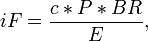 where
where
- iF = intake fraction (unitless after proper unit conversions)
- c = exposure concentratíon of the population (µg/m3)
- P = population size
- BR = breating rate, usually a nominal value 20 m3/d is used
- E = emission of fine particles (g/s)
In an assessment, exposure concentration c is solved from the equation and used as exposure in health impact modelling.
Rationale
Inputs and calculations
Variables used to calculate exposure in an assessment model (in µg/m3 in ambient air average concentration).
| Variable |
Measure |
Indices |
Missing data
|
| emissions (from the model) is in ton /a
|
|
Required indices: - . Typical indices: Time, City_area, Exposure_agent, Emission_height.
|
|
| iF (generic data but depends on population density, emission height etc)
|
conc (g /m3) * pop (#) * BR (m3 /s) / emis (g /s) <=> conc = emis * iF / BR / pop # conc is the exposure concentration
|
Required indices: - . Typical indices: Emission_height, Area
|
|
| population
|
Amount of population exposed.
|
Required indices: - . Typical indices: Time, Area
|
|
Data
These data come from
[29]
Pollutants:
- PM10-2.5: Primary PM10 - primary PM2.5
- PM2.5: Primary PM2.5
- SO2: Secondary PM2.5 derived from SO2 (in practice, SO_4)
- NOx: Secondary PM2.5 derived from NOx (in practice, NO_3)
- NH3: Secondary PM2.5 derived from NH3 (in practice, NH4)
Intake fractions of PM(ppm)| Obs | Pollutant | Emission height | Urban | Rural | Remote | Average | Description |
|---|
| 1 | PM10-2.5 | High | 8.8 | 0.7 | 0.04 | 5.0 | |
| 2 | PM10-2.5 | Low | 13 | 1.1 | 0.04 | 7.5 | |
| 3 | PM10-2.5 | Ground | 40 | 3.7 | 0.04 | 23 | |
| 4 | PM10-2.5 | Average | 37 | 3.4 | 0.04 | 21 | |
| 5 | PM2.5 | High | 11 | 1.6 | 0.1 | 6.8 | |
| 6 | PM2.5 | Low | 15 | 2.0 | 0.1 | 6.8 | |
| 7 | PM2.5 | Ground | 44 | 3.8 | 0.1 | 25 | |
| 8 | PM2.5 | Average | 26 | 2.6 | 0.1 | 15 | |
| 9 | SO2 | | 0.99 | 0.79 | 0.05 | 0.89 | |
| 10 | NOx | | 0.2 | 0.17 | 0.01 | 0.18 | |
| 11 | NH3 | | 1.7 | 1.7 | 0.1 | 1.7 | |
Exposure-response functions of environmental pollutants
Question
What are the exposure-response functions (ERF) of environmental pollutants that do not have own pages in Opasnet?
Answer
Exposure-response function (ERF) is a mathematical quantitative description of the relationship between an exposure to an agent and the health responses it causes in the human body. How to actually estimate the responses based on ERF is described in detail on page Health impact assessment.
Relevant example results can be found from here (in Finnish).
Rationale
Data
Helsinki energy decision 2015 methods(-)| Obs | Exposure agent | Response | Subgroup | Exposure | ER function | Scaling | Exposure unit | Threshold | ERF | Description |
|---|
| 1 | Indoor radon | Lung cancer morbidity | | Annual average indoor air concentration | RR | None | Bq /m3 | 0 | 1.0016 (1.0005-1.0031) | |
| 2 | Chlorination byproducts | Bladder cancer morbidity | | Concentration in ingested water | RR | None | µg /l | 0 | 1.0039 (1.00053-1.00722) | |
| 3 | Chlorination byproducts | Bladder cancer morbidity | | Concentration in ingested water | RR | None | netrev /l | 0 | 1.000029 (1-1.000072) | |
| 4 | Arsenic | Bladder cancer morbidity | | Concentration in ingested water | RR | None | µg /l | 0 | 1.002 (0.999-1.006) | |
| 5 | Formaldehyde | Asthma morbidity | Age:<14 | Annual average indoor concentration | RR | None | µg /m3 | 0 | 1.0140743178 | |
| 6 | Formaldehyde | Asthma morbidity | Age:>=14 | Annual average indoor concentration | RR | None | µg /m3 | 0 | 1 | |
| 7 | Dampness damage | Asthma morbidity | | Yes/no moisture damage | RR | None | % | 0 | 1.37 (1.23-1.53) | |
| 8 | Dampness damage | Lower respiratory symptoms morbidity | | Yes/no moisture damage | RR | None | % | 0 | 1.5 (1.38-1.86) | |
| 9 | Dampness damage | Upper respiratory symptoms morbidity | | Yes/no moisture damage | RR | None | % | 0 | 1.7 (1.44-2) | |
| 10 | Fluoride | Fluorosis | Age:<14 | Concentration in ingested water | UR | None | | 0 | 0.125 | |
| 11 | Fluoride | Fluorosis | Age:>=14 | Concentration in ingested water | UR | None | | 0 | 0 | |
| 12 | Lead | Decrease of IQ below 70 points | | Intake level from food | UR | None | ? | 0 | 0.025 | |
| 13 | Lead | Increased blood pressure | | Intake level from food | UR | None | ? | 0 | 0.025 | |
| 14 | Lead | IQ loss | Age:Age 1 | Blood concentration | UR | None | IQ l /ug | 24 | 0.039 (0.024 - 0.053) | Lanphear et al 2005 https://doi.org/10.1289/ehp.7688 using the first increment from 24 to 100 ug/l. Assumes threshold at 24 ug/l although this is strong assumption |
| 15 | Aflatoxin | Liver cancer | Hepatitis:Hepatitis B- | Intake via food | UR | None | # /(ng /kg /d /100000py) | 0 | 0.01 (0.002 - 0.03) | WHO. Is this per year or per lifetime? |
| 16 | Aflatoxin | Liver cancer | Hepatitis:Hepatitis B+ | Intake via food | UR | None | # /(ng /kg /d /100000py) | 0 | 0.3 (0.01 - 0.5) | WHO. Is this per year or per lifetime? |
| 17 | Formaldehyde | Nasal cancer morbidity | | Annual average indoor concentration | UR | None | µg /m3 | 0 | 0.000013 | |
| 18 | Benzene | Leukemia morbidity | | Annual average indoor concentration | UR | None | µg /m3 | 0 | 0.000005 | |
| 19 | Quatzdust | Silicosis morbidity | | Indoor air concentration | UR | None | mg /m3 | 0 | 0.125; 0.125; 0.25 | |
| 20 | Asbestos at work | Lung cancer and mesothelioma morbidity | | Indoor air concentration | UR | None | | 0 | 0.05 (0.01-0.1) | |
| 21 | Noise at work | Hearing damage | | Noise level | UR | None | | 0 | 570 | Medium noise (80-85 dB) |
| 22 | Noise at work | Hearing damage | | Noise level | UR | None | | 0 | 1320 | Loud noise (>85 dB) |
Ozone and PM2.5 moved to ERF of outdoor air pollution.
Calculations
External cost
External costs are costs that are not included in the price of a product but still cause negative (or sometimes positive) impacts to the society or stakeholders. The market theory says that if external costs cannot be included in prices e.g. using taxation, the market process will lead to outcomes that deviate from the societal optimum.
Question
What are important external costs in environmental health?
Answer
Health impacts and climate impacts are often not considered in pricing, so they remain as external costs. The code below is used to fetch the variable for models.
Rationale
Numbers are rough estimates based on typical health impact assessments and common target prices of carbon trade.
References
- ↑ Helsingin ympäristötilasto. Helsingin kaupungin ympäristökeskus. http://www.helsinginymparistotilasto.fi/
- ↑ Scanoffice.fi: VTT:n testiraportit - Ilmalämpöpumppuvertailu. http://www.scanoffice.fi/fi/tuotteet/tuoteryhmat/ilmalampopumput/raportit-ja-sertifikaatit/vttn-testiraportit
- ↑ Energy.gov: Geothermal heat pumps. U.S. department of energy. http://energy.gov/energysaver/geothermal-heat-pumps
- ↑ Energy.gov: Wood and pellet heating. U.S. department of energy http://energy.gov/energysaver/wood-and-pellet-heating
- ↑ Norwegian Water Resources and Energy Directorate: Energy in Norway, an brief annual presentation, 2009. http://www.nve.no/global/energi/analyser/energi%20i%20norge%20folder/energy%20in%20norway%202009%20edition.pdf
- ↑ Sustainable Energy Technology at Work -project: Use of waste heat from refining industry, Sweden. Preem AB, H Samuelsson. http://www.setatwork.eu/database/products/R179.htm
- ↑ Berntsson T, Persson Elmeroth L, Algehed J, Hektor E, Franck PÅ, Åsblad A, Johnsson F, Lyngfelt A, Gevert B, Richards T: Towards a Sustainable Oil Refinery - Pre-study for larger co-operation projects. Chalmers Energy Centre (CEC) Report 2008:1. Chalmers University of Technology. http://publications.lib.chalmers.se/records/fulltext/69752.pdf
- ↑ Ilkka Maaskola, Matti Kataikko: Ylijäämälämmön taloudellinen hyödyntäminen. Lämpöpumppu- ja ORC-sovellukset. Motiva, Helsinki, 2014. http://www.motiva.fi/files/10217/Ylijaamalammon_taloudellinen_hyodyntaminen_Lampopumppu-_ja_ORC-sovellukset.pdf
- ↑ Helen: Lisäämme tuulivoimalla tuotetun energian määrää. https://www.helen.fi/kotitalouksille/neuvoa-ja-tietoa/vastuullisuus/hiilineutraali-tulevaisuus/lisaa-tuulivoimaa/
- ↑ Helen: Aurinkovoiman tuotanto on käynnistynyt Suvilahdessa. 10.3.2015 https://www.helen.fi/uutiset/2015/aurinkovoiman-tuotanto-on-kaynnistynyt-helsingin-suvilahdessa/
- ↑ Loviisan sanomat: Loviisan ydinvoimalan tehoja aiotaan nostaa 52 megawattia. 13.1.2012 http://www.loviisansanomat.net/lue.php?id=5361
- ↑ Valtioneuvoston periaatepäätös Loviisa 3 -ydinvoimalasta. 6.5.2010 https://www.tem.fi/files/26809/PAP_FPH_LO3.pdf
- ↑ Lähdeaho Marika, Meskanen Jukka, Yrjänäinen Heli: Sähköenergian kustannusrakenne: vertailuna vesivoima, hiilivoima ja ydinvoima. Seminaarityö. Tampere university of technology. http://www.tut.fi/smg/tp/kurssit/SMG-4050/seminaarit07/sahkoenergian_kustannusrakenne.pdf
- ↑ Krohn S (editor), Morthorst PE, Awerbuch S: The Economics of Wind Energy. European Wind Energy Association (EWEA). March 2009 [http://www.ewea.org/fileadmin/files/library/publications/reports/Economics_of_Wind_Energy.pdf
- ↑ Vainio Tuukka: Sähkön tuotantokustannusvertailu. Aalto-yliopisto, Insinööritieteiden korkeakoulu, energiatekniikan laitos. 2011 https://aaltodoc.aalto.fi/bitstream/handle/123456789/4969/isbn9789526041353.pdf?sequence=1
- ↑ Hawkings, Will: An affordable district heating system in Norway. Heat Pupms Today. 10.3.2014 http://www.heatpumps.media/features/an-affjordable-district-heating-system-in-norway
- ↑ Kenneth Hoffmann MSc, David Forbes Pearson MInstR: Ammonia Heat Pumps for District Heating in Norway – a case study. The Institute of Refrigeration (IOR). 2011 http://www.ammonia21.com/web/assets/link/Hoffman7thApril2011London%20colour.pdf
- ↑ European Heat Pump Association: The World's Largest “Natural” District Heat Pump. 6.3.2015 http://www.ehpa.org/about/news/article/the-worlds-largest-natural-district-heat-pump/
- ↑ Lako, Paul: Geothermal heat and power. Energy technology systems analysis programme, IEA. 2010. http://www.etsap.org/E-techDS/PDF/E06-geoth_energy-GS-gct.pdf
- ↑ Helen Oy: Lämpölaitosten turvallisuustiedote. 17.6.2015 https://www.helen.fi/globalassets/ymparisto/turvallisuustiedote-lampolaitokset.pdf
- ↑ Lehtilä A, Koljonen T, Airaksinen M, Tuominen P, Järvi T, Laurikko J, Similä L, Grandell L: Energiajärjestelmien kehityspolut kohti vähähiilistä yhteiskuntaa. Low Carbon Finland 2050 -platform. VTT. 2014. http://en.opasnet.org/en-opwiki/images/d/d1/Low_Carbon_Finland_Platform.pdf
- ↑ Tilastokeskus (Statistics Finland). List of tables under the topic "Price of energy". http://pxweb2.stat.fi/database/statfin/ene/ehi/ehi_fi.asp
- ↑ U.S. Energy Information Administration: Spot prices for crude oil and petroleum products. http://www.eia.gov/dnav/pet/PET_PRI_SPT_S1_A.htm
- ↑ Internal revenue service: Nonconventional Source Fuel Credit, Inflation Adjustment Factor, and Reference Price http://www.irs.gov/pub/irs-drop/n-99-18.pdf
- ↑ U.S. Energy Information Administration: Annual Energy Outlook 2015 - With Projections to 2040. 2015. http://www.eia.gov/forecasts/aeo/pdf/0383(2015).pdf
- ↑ Tilastokeskus (Statistics Finland): Energian hinnat 2015, 1. vuosineljännes. (Energy prices 2015, 1. quarter) http://tilastokeskus.fi/til/ehi/2015/01/
- ↑ Väisänen S: Greenhouse gas emissions from peat and biomass-derived fuels, electricity and heat - Estimation of various production chains by using LCA methodology. Lappeenranta University of Technology. 2014. http://www.doria.fi/bitstream/handle/10024/94404/isbn9789522655578.pdf?sequence=2
- ↑ http://www.ymparisto.fi/download.asp?contentid=3706 ⇤--#: . Link broken. I simply don't know what this is supposed to be. --~~~~ (type: truth; paradigms: science: attack)
- ↑ 29.0 29.1 Sebastien Humbert, Julian D. Marshall, Shanna Shaked, Joseph V. Spadaro, Yurika Nishioka, Philipp Preiss, Thomas E. McKone, Arpad Horvath, and Olivier Jolliet. Intake Fraction for Particulate Matter: Recommendations for Life Cycle Impact Assessment (2011). Environmental Science and Technology, 45, 4808-4816.