Evaluation of intake fractions for different subpopulations due to primary fine particulate matter (PM2.5) emitted from domestic wood combustion and traffic in Finland

This page is a nugget. The page identifier is Op_en5557
Moderator:Essi Vuorinen (see all)
Upload data	Unlike most other pages in Opasnet, the nuggets have predetermined authors, and you cannot freely edit the contents. Note! If you want to protect the nugget you've created from unauthorized editing click here

This page (including the files available for download at the bottom of this page) contains a draft version of a manuscript, whose final version is published and is available in the Air quality, atmosphere & health. If referring to this text in scientific or other official papers, please refer to the published final version as: Pauliina Taimisto, Marko Tainio, Niko Karvosenoja, Kaarle Kupiainen, Petri Porvari, Ari Karppinen, Leena Kangas, Jaakko Kukkonen, Jouni T. Tuomisto: Evaluation of intake fractions for different subpopulations due to primary fine particulate matter (PM2.5) emitted from domestic wood combustion and traffic in Finland. Air quality, atmosphere & health. Received: 29 October 2009 / Accepted: 8 February 2011 (c) Springer Science+Business Media B.V. 2011 doi:10.1007/s11869-011-0138-3 .

Title

Editing Evaluation of intake fractions for different subpopulations due to primary fine particulate matter (PM2.5) emitted from domestic wood combustion and traffic in Finland

Authors and contact information

Pauliina Taimisto, correspondence author

(pauliina.taimisto@thl.fi

(National Institute for Health and Welfare (THL), Kuopio, Finland)

Marko Tainio

(National Institute for Health and Welfare (THL), Kuopio, Finland)

(Systems Research Institute, Polish Academy of Sciences, Warsaw, Poland)

Niko Karvosenoja

(Finnish Environment Institute, Helsinki, Finland)

Kaarle Kupiainen

(Finnish Environment Institute, Helsinki, Finland)

Petri Porvari

(Finnish Environment Institute, Helsinki, Finland)

Ari Karppinen

(Finnish Meteorological Institute, Helsinki, Finland)

Leena Kangas

(Finnish Meteorological Institute, Helsinki, Finland)

Jaakko Kukkonen

(Finnish Meteorological Institute, Helsinki, Finland)

Jouni T. Tuomisto

(National Institute for Health and Welfare (THL), Kuopio, Finland)

Abstract

Domestic wood combustion and traffic are the two most significant primary fine particulate matter (PM_2.5) emission source categories in Finland. We estimated emission–exposure relationships for primary PM_2.5 emissions from these source categories using intake fractions (iF), which describes the fraction of an emission that is ultimately inhaled by a target population. The iFs were calculated for four different emission source subcategories in Finland in 2000: (1) domestic wood combustion in residential buildings, (2) domestic wood combustion in recreational buildings, (3) traffic exhaust and wear emissions, and (4) traffic resuspension emissions. The iFs were estimated for both total population and for subpopulations with different gender, age, and educational status. Primary PM_2.5 emissions were based on the Finnish Regional Emission Scenario model and the dispersion of particles was calculated using the Urban Dispersion Modeling system of Finnish Meteorological Institute. Both emissions and dispersion were estimated on a 1 km spatial resolution. The iFs for primary PM_2.5 emissions from (1) residential and (2) recreational buildings were 3.4 and 0.6 per million, respectively. The corresponding iF for (3) traffic exhaust and wear and (4) traffic resuspension emissions were 9.7 and 9.5 per million, respectively. The differences in population-weighted outdoor concentrations were significant between subpopulations with different educational status so that people with higher education were exposed more to traffic-related PM_2.5.

Keywords

iF, Intake fraction, Exposure, Particulate matter, Domestic combustion, Traffic

Introduction

Exposure to air pollution, especially for fine particulate matter (PM2.5; particles with aerodynamic diameter of less than _2.5 μm), have been associated with increases in mortality and hospital admissions due to respiratory and cardiovascular diseases (Dockery et al. 1993; Pope et al. 2002; WHO 2003; Beelen et al. 2008; Brunekreef and Holgate 2002). The Clean Air for Europe program have estimated that PM_2.5 is associated with more than 348,000 premature deaths and to loss of nearly 3.7 Ma of life in Europe in 2000 (Watkiss et al. 2005). The other study, based on measured PM concentrations, estimated that PM_2.5 air pollution causes 492,000 premature deaths and loss of 4.9 Ma of life lost in Europe in 2005 (de Leeuw and Horàlek 2009).

In Finland, an integrated assessment model for primary PM_2.5 air pollution has been developed to estimate emissions, dispersion, and adverse health effects of primary PM_2.5 air pollution (Kukkonen et al. 2008; Kauhaniemi et al. 2008). In a previous assessment of the present authors, dispersion and exposure of primary PM2.5 were evaluated in Finland using regional scale dispersion model system SILAM (Sofiev et al. 2006) on the spatial resolution of approximately 5 km (Tainio et al. 2009a) and the adverse health effects were estimated for the whole population (Tainio et al. 2010). The primary PM_2.5 emissions from Finland were concluded to cause annually approximately 179 premature deaths in Finland (Tainio et al. 2010). Over half of the deaths were associated with domestic wood combustion and traffic emissions from Finland.

One of the main conclusions of Tainio et al. (2009a) was that the emission–exposure calculations for emission sources with low emission height, such as traffic and domestic wood combustion, need to be refined. Traffic emissions occur to considerable extent in densely populated urban environments, while the wood combustion emissions occur both in rural and in urban environments. This has been illustrated in a study where the vicinity of primary PM_2.5 emissions and population was evaluated over Finland (Tainio et al. 2009b).

Karvosenoja et al. (2010) compared population exposure effects of traffic and domestic wood combustion using two different source-receptor dispersion matrix set-ups: (1) identical to this study on the horizontal grid resolution of 1 km, and (2) based on the SILAM atmospheric model identical to Tainio et al. (2009a) on the resolution of 10 km. The study pointed out the benefits of using finer spatial resolution for low-altitude emissions especially in the vicinity of high population densities.

Intake fraction describes the fraction of a pollutant released from source and summed over exposed individuals and divided by the emission (Bennett et al. 2002). It has been used in a substantial number of air pollution studies (e.g., Levy et al. 2002a; Greco et al. 2007). For example, Stevens et al. (2007) have used the iF concept to compare different exposure assessment methods with each other in Mexico City due to PM_2.5 emissions from mobile sources. In that study, the iFs for primary PM_2.5 varied from 23 to 120 per million depending on the method used.

Different subpopulations have different exposure levels. This could be a result of living in different locations (e.g., families with children might live in different areas than the elderly) or due to differences in time activity (e.g., adults may spend more time in traffic than other subpopulations). In previous studies, Levy et al. (2002b) have estimated that people with higher education have lower premature mortality due to air pollution. Greene and Morris (2006) evaluated the health risks of PM_2.5 for different subpopulations and concluded that females and adults had highest lifetime risks for developing new lung cancer cases due to PM_2.5. Beelen et al. (2008) concluded that population with lower education had higher adverse health effects due to traffic air pollution.

In this study, we estimated emission–exposure relationships for primary PM_2.5 emissions due to domestic wood combustion and traffic in Finland in 2000. Although, for simplicity, concepts such as “emission–exposure relationship” are used throughout this article, strictly speaking, the term “exposure” refers here to population-weighted outdoor concentrations (of PM_2.5). The emissions and atmospheric dispersion were estimated on a finer spatial resolution of 1 km. The emission–exposure relationships for both domestic wood combustion and traffic were evaluated for two emission source subcategories. We also estimated emission– exposure relationships and the population-weighted outdoor concentrations for subpopulations with different gender, age, and educational status.

Material and methods

Emissions

Primary PM_2.5 emissions of domestic wood combustion and road traffic were calculated with the Finnish Regional Emission Scenario (FRES) model of the Finnish environment institute (Karvosenoja et al. 2008). The emissions of primary PM_2.5 are calculated by combining (1) activity levels, (2) emission factors, and (3) emission control technologies (for detailed description of these parameters, see Karvosenoja et al. 2008). The basic spatial and temporal domains of the model are Finland and 1 year, respectively, which are then disaggregated to 1 km and 1 h resolutions, respectively. The 1 km and hour resolutions were used in the dispersion computations (see below). The national level emission calculation and data sources for traffic exhaust and domestic wood combustion are presented in Karvosenoja et al. (2008), and for traffic non-exhaust in Kupiainen et al. (2007). The basis for the spatial and temporal allocations of emissions are presented in detail in Karvosenoja et al. (2010). The description of emission source categories and subcategories are presented in Tables 1 and 2.

Domestic wood combustion and traffic emissions are calculated separately for various wood combustion appliance and vehicle types, direct wear products of road, tires and brakes, and particle resuspension from road surfaces. In this paper emissions are presented aggregated to four categories based on their different temporal variations: (1) wood heating in residential buildings, (2) wood heating in recreational buildings (3) traffic exhaust and wear, and (4) resuspension from road surfaces. The temporal disaggregation in time was carried out using typical temporal patterns based on data from wood use and traffic surveys. Wood combustion emissions from residential buildings are highest during winter, whereas for recreational buildings the maximum occurs during non-winter months. Hourly maximum of wood combustion emissions occurs at early evening hours. For exhaust traffic emissions, monthly variation is less pronounced, and for resuspension emissions, the maximum occurs during winter and spring months (Kupiainen 2007). Traffic emissions have their maximum during the morning and afternoon rush hours, and also the lower emissions during weekends are taken into account.

Atmospheric dispersion

The dispersion of primary PM_2.5 was evaluated with the Urban Dispersion Modeling system (UDM-FMI) developed at the Finnish Meteorological Institute (Karppinen et al. 2000a, b). It includes a multiple source Gaussian plume model and a meteorological pre-processor MPP-FMI (Karppinen et al. 1997, 1998). For the selected calculation grid, the system can be used to compute an hourly time series of concentrations. The parameters used in dispersion calculations are presented in Table 2.

The MPP-FMI model uses synoptic weather observations and meteorological soundings, and its output consists of hourly time series of meteorological parameters, including atmospheric turbulence parameters and the mixing height of the atmospheric boundary layer. In order to have input data representative for different areas in Finland, meteorological observations from ten synoptic weather stations were used in the calculations. The stations selected were Helsinki, Turku, Lappeenranta, Jokioinen, Kankaanpää, Jyväskylä, Kuopio, Oulu, Rovaniemi, and Sodankylä. The corresponding sounding observations were taken from the Jokioinen and Sodankylä observatories.

In this study, the UDM-FMI model was used to calculate source-receptor matrices. These matrices describe the dispersion of inert particles from a single emission source of unit strength, and they are combined with the actual emissions to compute the PM_2.5 concentrations. The size of the unit source was set at 1×1 km2, corresponding to the resolution of the emission inventory. The source was assumed to be in the center of a square calculation grid of size 40×40 and 20×20 km² for domestic wood combustion and traffic emissions, respectively. The size of the domain was chosen so that it covers most of the substantially elevated concentrations from both categories of sources. Detailed numerical computations show that the computational domain includes at least 85% and 90–95% of the pollutant mass for wood combustion and traffic emissions, respectively. The diurnal and seasonal variations of the emissions were taken into account, as described above. Removal of particles through deposition was neglected, due to the relatively small particle size and the short time scales considered.

The source-receptor matrices were computed for four different emission source subcategories (Table 1). The differences between the various emission categories were the different seasonal and diurnal variation of the emissions, and varying source heights (Table 2). The emission heights including the estimated initial plume rises were assumed to be 7.5 and 2.0 m for domestic wood combustion and traffic, respectively. The concentrations were calculated at the height of 2.0 m. The dispersion matrices were calculated from hourly concentrations as annual averages for the year 2000, for the ten stations mentioned above, and for the above mentioned four emission categories, i.e., altogether 40 matrices were computed.

Table 1. Description of emission source categories and subcategories used in this study

Source category	Traffic		Domestic wood combustion
Subcategory	Traffic exhaust and wear	Traffic resuspension	Residential buildings	Recreational buildings
Description of source subcategory	Primary PM2.5 emissions from traffic exhaust and direct wear emissions from road, tires and brakes	Primary PM2.5 emissions caused by particle resuspension from road surfaces	Primary PM2.5 emissions from primary and supplementary wood heating in residential buildings	Primary PM2.5 emissions from wood heating in recreational buildings

Table 2. Parameters of emission source categories and subcategories for primary PM_2.5 used in this study

Source category	Traffic		Domestic wood combustion
Subcategory	Traffic exhaust and wear	Traffic resuspension	Residential buildings	Recreational buildings
Emission strength (whole of Finland) (g/s)	146	88	198	40
Spatial resolution of emissions and source-receptor matrices (km)	1	1	1	1
Emission height including initial plume rise (m)	2	2	7.5	7.5
Dispersion domain used in the SRM computations (km2)	20×20	20×20	40×40	40×40

There are differences between matrices especially between different stations, due to varying meteorological conditions, e.g., prevailing wind direction and speed. There are also differences between the matrices for traffic and wood combustion emissions, due to varying release heights. Traffic emissions have lower release height, and therefore concentrations in the center of the calculation area are higher than for domestic wood combustion. Different seasonal variation between the emission subcategories also results in some differences in dispersion patterns. Some examples of sourcereceptor matrices are given in Figs. 1 and 2 to illustrate the different dilution of the emission for different cases. The effect of different meteorological conditions between stations is depicted in Fig. 1a–b. An example of differences in dispersion due to different seasonal variation of emissions is given in Fig. 2a–b for domestic wood combustion— emissions from residential buildings are highest in winter, whereas emissions from recreational buildings have their maximum during non-winter months, which results in a different dispersion pattern.

The matrices were combined with the data regarding the spatial distribution of emissions to calculate the concentration levels due to nearby emissions of wood combustion and road traffic for the whole of Finland. Each emission value was multiplied with the appropriate value from the source-receptor matrix, and the resulting concentration fields were summed up. For most cases, the sourcereceptor matrix of the nearest station was used, with two exceptions. The border between Oulu and Rovaniemi, as well as in southern Finland the border between the effect of coastal stations (Helsinki and Turku) and inland stations, were redefined in order to achieve a better compliance with the borders of the climatic zones.

Fig. 1 An example of sourcereceptor matrices for different stations. Matrices for resuspened traffic emissions for Kuopio and Rovaniemi for the year 2000. Concentration of PM in micrograms per cubic meter assuming a source of size 1×1 km² and strength of 1,000 kg/a in the centre of the calculation area

Fig. 2 An example of source- b) receptor matrices for different source categories. Matrices for emissions from residential and recreational buildings for Helsinki for the year 2000. Concentration of PM in micrograms per cubic meter assuming a source of size 1×1 km2 and strength of 1,000 kg/a in the centre of the calculation area

Population

The population data were provided by the Statistics Finland Grid Database (http://www.stat.fi/tup/ruututietokanta/ index_en.html). The dataset contained population numbers for Finland on a resolution of 250×250 m² for 2004. The same population data were used also in Tainio et al. (2009a). In addition to population densities of the total population, the dataset contained population densities for subpopulations with different gender, age, and educational status (Table 3). The population data were combined with the concentration data so that population numbers of each grid were joined to the nearest concentration point. The joining of data was done with the ArcMap version 9.2 (http://www.esri.com/)

Table 3. The description of subpopulations with different age, gender and educational status as used in the calculations

Subgroup	Description	Population
Female	Female	2,664,334
Male	Male	2,539,492
Children (0–17)	Children between 0 and 17 years old	1,094,751
Adults (18–64)	Adults between 18 and 64 years old	3,272,098
Elderly (65–)	People over 64 years old	836,977
Higher education	People with an academy level education, and graduate school levels	570,267
High school	People with matriculation	325,831
Vocational education	People with middle level education, excluding matriculation	1,793,804
Comprehensive school	People without education after comprehensive school level, or it is unknown	1,398,225
All	Total population in Finland	5,203,826

Emission–exposure relationship

The emission–exposure relationships for different primary PM2.5 emission source categories and subcategories were estimated using intake fraction (iF) concept (Bennett et al. 2002). The iF is the fraction of an emission of a pollutant that is inhaled by the population (Bennett et al. 2002). The intake fraction iFs were calculated with Eq. 1:

$\frac{iF_{s,i,j}=\sum(c_{s,i}*Pop_{i,j}*BR)}{Q_s}$

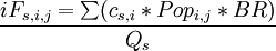
where

$Q_s$ is the total emission from the emission source category or subcategory s

$c_{s,i}$ is the incremental outdoor concentration of PM (grams per cubic meter) in a grid cell $i (i=1..n,$ where $n$ is the total number of grid cells), caused by $Q_s$

$Pop_{i,j}$ is the population size in the grid cell $i$ for subpopulation $j$

$BR$ is the average individual breathing rate. A nominal breathing rate of 20 m³ day⁻¹ person⁻¹ (∼0.00023 m³ s⁻¹person⁻¹) was adopted in this study. We used the same breathing rate for all subpopulations resulting differences in spatial distribution.

The total number of grid cells for the whole Finland (i) was 783,900. The population–weighted outdoor concentration of PM_2.5 was used as a proxy for the population exposure while calculating the iFs. The multiplying of population numbers with PM_2.5 concentrations (C×Pop in Eq. 1) was done with ArcMap version 9.2 and rest of the iF calculations with statistical computation and graphic system R version 2.7.0 (The R Foundation for Statistical Computing, http://www.r-project.org/).

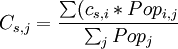
Population–weighted outdoor concentration

The population–weighted outdoor concentrations of PM_2.5 was estimated with Eq. 2:

$C_{s,j}=\frac{\sum(c_{s,i}*Pop_{i,j}}{\sum_jPop_j}$

where

$C_{s,i,j} =$ population–weighted outdoor concentration for primary PM2.5 for sector s and for subpopulation $j$ (grams per cubic meter)

$c_{s,i}$ is the incremental outdoor concentration of PM (grams per cubic meter) in a grid cell $i (i=1..n,$ where $n$ is total number of grid cells), caused by $Q_s$

$Pop_{i,j}$ is the population size in the grid cell i for subpopulation $j$.

Results

Fig. 3 Population–weighted outdoor PM_2.5 concentrations (micrograms per cubic meter) of different subpopulations in Finland for primary PM_2.5 emissions due to traffic and domestic wood combustion in 2000. See Table 3 for description of different subpopulations

Fig. 4 The iFs for Finnish primary PM_2.5 emissions from traffic and domestic wood combustion for different emission source subcategories and subpopulations in Finland in 2000. The relative differences compared with exposures (Fig. 3) are due to the subpopulation sizes. See Table 3 for description of different subpopulations

The iFs for primary PM_2.5 emissions originated from domestic wood combustion and traffic in Finland in 2000 were 2.9 and 9.6 per million, respectively (Table 4). The iFs for the combined traffic exhaust and wear emissions, and traffic resuspended emissions were 9.7 and 9.5 per million, respectively. The small difference in iF values between these two emission source subcategories was due to relatively higher exhaust emissions in urban driving conditions.

The iFs for domestic wood combustion for residential buildings and for recreational buildings were 3.4 and 0.6 per million, respectively (Table 4). The difference in iF shows that the PM_2.5 emissions from these two subcategories expose the population in a substantially different efficiency. A practical implication of this result is that the emission reduction of primary PM2.5 from residential buildings has a relatively larger impact on exposure and health, compared with the corresponding emission reductions in recreational buildings.

The population–weighted outdoor concentration of the different population subgroups for primary PM_2.5 emissions from domestic wood combustion and traffic are presented in Fig. 3a–c. The corresponding iFs are presented in Fig. 4a–c. The population–weighted outdoor concentrations of PM_2.5 did not have significant relative differences between populations with different gender and age status. In subpopulations with different educational status, the average concentrations varied between 1.1–1.7 and 0.7– 1.0 μg/m³ for traffic exhaust and wear, and traffic resuspensed emissions, respectively so that people with higher education had higher average concentrations than people with lower education (Fig. 3c). There were no significant differences between different educational statuses in population–weighted outdoor concentration of PM2.5 air pollution due to domestic wood combustion.

The differences of the iF values between subpopulations were higher than those for the population–weighted outdoor concentrations (Fig. 4a–c). These differences can be explained mainly by the size variations of the different subpopulations (Table 3), as these iF values are defined as the fraction of emission inhaled by all members of the population subgroup (see Eq. 1).

Table 4. Comparison of the estimated intake fractions (iF) corresponding to the emissions of primary PM_2.5 from Finland, between the present study and Tainio et al.’s (2009a) study

Emission source category	Subcategory	Intake fraction (per million)
		The present study	Tainio et al.’s (2009a) study
Traffic	Alla	9.6	0.7
	Traffic exhaust and wear	9.7
	Traffic resuspended	9.5
Domestic combustion	Allb	2.9	0.5
	Residential building	3.4
	Recreational buildings	0.6

Tainio et al. (2009a) used the same emission and population data, but a different dispersion model. See Table 5 for details. We have compared

only the results regarding the same spatial area (Finland) and population (in Finland)

^a The iF value estimated in Tainio et al. (2009a) for traffic includes the emissions of tailpipe and direct wear emissions from road, tires, and brakes and

traffic resuspended emissions

^b The iF value estimated in Tainio et al. (2009a) for domestic combustion includes the emissions from both the residential and recreational wood

combustion

Table 5. Comparison of input data and methods between the present study and Tainio et al.’s (2009a) study

Input	The present study	Tainio et al.’s (2009a) study
Domain	Finland	Europe and Finland (the latter using a finer resolution)
Emission data	FRES	FRES for Finland, EMEP for the whole of Europe
Emission source categories	4 source categories for traffic and domestic wood combustion (including subcategories for both)	6 source categories including traffic and domestic wood combustion
Dispersion model	UDM-FMI (urban and local scale dispersion model)	SILAM (regional and continental scale ispersion model)
Meteorology	MPP-FMI (meteorological preprocessing model, input data from synoptic weather observations and soundings)	FMI variant of HIRLAM (numerical weather prediction model)
Dispersion domain	Square of size 20×20 km2 or 40×40 km2	Europe, or Finland and nearby areas
Source size for area e missions	1×1 km2	30×30 km2 for Europe and 5×5 km2 for Finland
Vertical mixing	Emission height 2.0 m (traffic) or 7.5 m (domestic combustion) including initial plume rise, statistical concentration distribution	Emission mixed to the whole boundary layer
Horizontal resolution of the results	1 km	30 km for Europe and 5 km for Finland
Exposed population	The population in Finland	The whole of Europe and the population in Finland
Breathing rate	20m3 day−1 person−1	20 m3 day−1 per person−1

Discussion

In this study we estimated iFs for primary PM_2.5 emissions due to traffic and domestic wood combustion in Finland in 2000. We found out that iF is higher for traffic-related primary PM_2.5 emissions than domestic wood combustion related primary PM_2.5 emissions. We also found out that the iF for residential building emissions is approximately six times higher than the iF for recreational building emissions. This difference is mainly caused by the much lower density of population near recreational buildings on the average than near other buildings with domestic combustion. These results show that primary PM_2.5 emission reduction from traffic sources reduces exposure more efficiently than emission reduction from domestic wood combustion, and emission reduction in residential buildings reduces exposure more efficiently than emission reduction in recreational buildings.

We also estimated population–weighted outdoor concentrations for different subpopulations to find out if there are substantial differences in exposure for primary PM_2.5 between subpopulations. We found out only minor differences in population–weighted outdoor concentrations between different subpopulations. The largest difference in concentrations was noted for PM_2.5 due to traffic and different education statuses so that average concentration for people with higher education was approximately 0.5 μg/m³ higher than average concentration for people with lower education. The results indicate that people with higher educational status live nearer traffic emission sources that other people. These results also imply that gender or age does not significantly affect the exposure of PM_2.5 due to low emission height sources.

Comparison of results to previous studies

The iFs calculated in this study are approximately an order of magnitude higher than iFs published in Tainio et al. (2009a) (Table 4). For traffic-related primary PM_2.5 emissions, the iF in present study was 9.6 per million and in Tainio et al. (2009a) 0.7 per million. For domestic wood combustion, the corresponding iFs were 2.9 per million and 0.5 per million, respectively. The iF for recreational buildings, 0.6 per million, is closer the iF value of 0.5 per million estimated in Tainio et al. (2009a). The present study and Tainio et al. (2009a) have several linkages in the methodology and data (see summary in Table 5). Both of these studies are based on primary PM_2.5 emission estimates made with FRES model and both use the same population data to estimate the population exposure. The main differences between the studies are the different meteorological and dispersion models and the resolution used in those models (Table 5).

The impact of horizontal grid resolution was studied in the Karvosenoja et al. (2010) article. The source-receptor matrices on the resolutions 1 and 10 km that were compared in Karvosenoja et al. (2010) were based on the same dispersion model as the present study and Tainio et al. (2009a), respectively. Based on the comparison, horizontal grid resolution is an important factor in describing differences between present study and Tainio et al. (2009a). However, also other factors, e.g., vertical mixing of emissions in the local and regional scale atmospheric models used, play a significant role (for a detailed discussion, see Karvosenoja et al. 2010).

Traffic

Several other studies have estimated emission–exposure relationships for PM_2.5 emissions due to traffic and wood smoke (Table 6). For traffic emissions, the published iFs varied from 0.7 per million (Tainio et al. 2009a) to 120 per million (Stevens et al. 2007). Most of the iF estimates are in between 5 and 10 per million. In this comparison, the iF values calculated in present study are slightly higher than iF values estimated elsewhere.

Highest iF values for traffic emissions are reported by Stevens et al. (2007). They compared five methods to estimate iF for PM_2.5 emissions due to traffic in Mexico City. The highest reported iF, 120 per million, was estimated with model that used inventory-particle composition method. In that model, iF was estimated from the measured primary PM_2.5 fraction, and the estimated primary PM_2.5 emissions if the chemical composition of PM_2.5 was known. The lowest iF in Stevens et al. (2007), 26 per million, was estimated with regression model that considers population within different distances from the emission source. Clearly, Mexico City is large city with several millions of inhabitants and high population density, and therefore iF estimates from there are expected to be clearly higher than iF values for traffic emissions in Finland.

The other studies published in US have reported iF values 1.2–9.4 per million (Greco et al. 2007; Marshall et al. 2005; Evans et al. 2002; Levy et al. 2002a). In NATA (National-scale Air Toxic Assessment) study, Marshall et al. (2005) reported population–weighted iF mean value of 4.4 per million for urban on-road traffic based diesel PM_2.5 emission sources among US urban counties. Marshall et al. (2005) used Assessment System for Population Exposure Nationwide (ASPEN) Gaussian plume dispersion model with meteorological data to estimate ambient concentrations, and probabilistic exposure model with ambient concentrations, time-activity information of population and differences between ambient and microenvironment exposure concentrations. For breathing rate they used 12 m3/day. The iF results for traffic emissions was half of the estimated iF for traffic in the present study. The results are not easily comparable because of model differences in emission category, areas, and breathing rate.

Greco et al. (2007) reported a value of 1.2 per million for primary PM_2.5 as median iF value for emissions of urban mobile source in the US. The result was based on a method where concentrations of ambient PM2.5 in the US were estimated by using a source-receptor matrix as a regressionbased derivation of output from the Climatological Regional Dispersion Model. In the source-receptor matrix they used database of transfer factors that summarized the impact of mobile sources of PM_2.5 and precursor emissions. Sourcereceptor matrix resolution was limited to county level. We estimated iF approximately eight times higher than was found in Greco et al. (2007).

Table 6 Selected intake fractions for traffic and domestic wood combustion PM_2.5 emissions

Source	iF (per million)	Geographical location	Method	Time scale	Breathing rate (m3/day)	Population characteristics	References
Traffic	120	Mexico City	iF method	–	20	Urban	Stevens et al. 2007
Traffic	26	Mexico City	iF method	–	20	Urban	Stevens et al. 2007
Traffic (exhaust and wear)	9.7	Finland	iF method	Year	20	People in country average	The present study
Traffic (resuspended)	9.5	Finland	iF method	Year	20	People in country average	The present study
Traffic	9.4	USA	CALPUFF	Year	12.2	Urban	Evans et al. 2002
Traffic	9.1	USA	CALPUFF	Year	20	Rural and urban	Levy et al. 2002a
Traffic	8.8	USA	CALPUFF	Year	12.2	Rural	Evans et al. 2002
Traffic	4.4	USA	NATA	Year	12.2	Urban	Marshall et al. 2005
Traffic	1.2	USA	S-R matrix	Year	20	County-level population	Greco et al. 2007
Traffic	0.7	Northern European	iF method	Year	20	People in country average	Tainio et al. 2009a
Wood smoke levoglucosan	15 (4.5–50)	Canada	iF methoda	Winter	14.5	Urban	Ries et al. 2009
Wood smoke	13 (6.6–24)	Canada	iF methoda	Winter	14.5	Urban	Ries et al. 2009
Wood smoke (residential buildings)	3.4	Finland	iF method	Year	20	People in country average	The present study
Wood smoke (recreational buildings)	0.6	Finland	iF method	Year	20	People in country average	The present study
Wood smoke (domestic combustion)	0.5	Northern European	iF method	Year	20	People in country average	Tainio et al. 2009a

The studies have been ordered primary between traffic and then domestic wood combustion studies and secondary from highest iF to lowest. Results from the present study are set in italics

^a Infiltration factor used in iF estimation

Domestic wood combustion

The emission–exposure relationship for the primary PM2.5 originated from domestic wood combustion (wood smoke) have been studied less extensively than those of traffic sources. Ries et al. (2009) used modeled data to estimate PM2.5 concentrations of residential wood smoke in Vancouver. Data were fit to monitor data for calm and cold winter periods. In addition, knowledge of estimation of residential wood burning emissions was used in iF evaluation. In the iF calculation, they used outdoor–indoor infiltration factor that made this evaluation different among all other iF studies, including ours. The iF result reported in Ries et al. (2009) was more than four times higher than in the present study.

Subpopulations

Exposure of different subpopulations to PM2.5 air pollution has been studied in EXPOLIS study based on measured population exposure in Helsinki Metropolitan Area, Finland (Rotko et al. 2000). They observed that less educated and young participants had greater exposures than more educated and older participants in the Helsinki metropolitan area (Rotko et al. 2000). Interestingly, our result is different. This is probably due to differences in study design. EXPOLIS directly studied personal exposures within a large city and thus included micro environmental and behavioral factors. Instead, our study did not assess these things, and all differences between subpopulations in our study are due to different home location patterns.

Health effect variation between subpopulations has been studied in several settings (Levy et al. 2002b; Kan et al. 2008; Beelen et al. 2008). For example, Kan et al. (2008) concluded in their epidemiological time-series analysis that females and the elderly were more vulnerable to outdoor air pollution. In general, these health studies proposed that the adverse effects of air pollution were higher with people with lower education compared with those with higher education. It is unclear if differences in the observed risks are due to exposure or sensitivity differences between subpopulations.

Model uncertainties

This study estimated exposures on the spatial resolution of 1 km. As was found out, this resolution resulted in much higher iF estimates for traffic and domestic wood combustion emissions than the previous Tainio et al. (2009a) study that used 5 km spatial resolution. In addition to different horizontal computation grid size, there are several other factors affecting the difference in the results obtained in the two studies, e.g., the vertical mixing in the two models used (Karvosenoja et al. 2010). However, it is likely that even a 1-km spatial resolution is too coarse to fully capture the exposure for these sources. A review done by Zhou and Levy (2007) concluded that the spatial extent of impact for traffic PM emissions is 100–400 m around the road. The review was done as meta-analysis by search of the peerreviewed literature and government reports focusing on air pollutants with study types of (bio)monitoring, air dispersion modeling, land use regression, and epidemiology.

Emission uncertainties for traffic and domestic wood combustion at country level have been assessed by Karvosenoja et al. (2008). The uncertainties were found to be considerable for traffic non-exhaust, i.e., resuspension and wear (the limits of the 95% confidence interval equals mean value minus 38% to the mean value plus 52%) and domestic wood combustion emissions (minus, 36% and plus, 50%), and less uncertain for traffic exhaust (±7%). Additional uncertainties caused by the spatial emission allocation have been qualitatively discussed by Tainio et al. (2009b).

The other uncertainty relates to population location. We assumed in this study that the home address represents the place where the population is exposed. However, people are, e.g., commuting from home to work and spend time in traffic. It is unclear how much this simplification affects the results of the present study.

The main uncertainty in the study relates to outdoor-toindoor transportation of the particles. We did not take this transportation into account in our calculations, but used outdoor concentration as proxy for exposure. This will overestimate calculated iF values, because only part of the PM_2.5 penetrates inside the buildings and we therefore overestimated the intake. There are considerable numbers of studies with estimates of home indoor–outdoor PM_2.5 concentrations (e.g., Hänninen et al. 2004; Molnar et al. 2005). For example, Hystad et al. (2009) have estimated residential infiltration efficiencies of outdoor PM_2.5 by using indoor–outdoor concentration measurements in Seattle, USA and Victoria, Canada. Also, Ries et al. (2009) used in iF calculations infiltration factor to account for outdoor-to-indoor effect as fraction of ambient PM_2.5 that penetrates indoors and remains resuspened.

Conclusions

The evaluation of emission–exposure relationships, expressed as intake fractions, showed that in Finland the traffic emissions expose people more efficiently than domestic wood combustion emissions. Also, the iF for residential emissions was six times higher than iF for recreational buildings. These results show that residential building emissions expose people more efficiently than recreational building emissions. Thus, emission reduction in residential building emission source category reduces the population exposure more efficiently than emission reduction in recreational building emissions. The population average exposure for the emissions from traffic and domestic wood combustion varied only slightly between different subpopulations. The only exception was the people with higher education, who were exposed more to the traffic emissions.

The iFs for traffic were over an order of magnitude higher in the present study compared with the corresponding values evaluated in the previous study by the same authors (Tainio et al. 2009b). The main differences between these two studies were the different dispersion models used, and the different horizontal spatial resolution, 1 and 5 km, respectively. Clearly, increasing the model resolution does not necessarily result in more accurate concentration results. The physical reason for this increase of the predicted exposure with finer model resolution is that the higher concentrations and the higher population densities are both spatially and temporally closely associated. An implication of this result is that the exposure values computed with fairly coarse resolution models (such as, e.g., regional scale models) can actually prove to be substantial underpredictions.

Acknowledgments

This study was performed as a part of the projects PILTTI (funded by the Ministry of the Environment, Finland, grant no. YM57/065/2005), INTARESE (funded by European Union, grant no. 018385–2), BIOHER (funded by Finnish Academy, grant no. 10155), MEGAPOLI (funded by European Union, FP/2007-2011, grant no. 212520), and Climate change, air quality and housing—future challenges to public health CLAIH (funded by Finnish Academy, grant no. 129355). This work was a part of the work in the Centre for Environmental Health Risk Analysis (jointly funded by the Academy of Finland, grants no. 53307, 111775, and 108571, and the National Technology Agency of Finland (Tekes) grant no. 40715/01). We would like to thank Mr. Kari Pasanen for his valuable help with ArcGis calculations.

References

Beelen R, Hoek G, van den Brandt P, Goldbohm R, Fischer P, Schouten L, Armstrong B, Brunekreef B (2008) Long-term exposure to traffic-related air pollution and lung cancer risk. Epidemiology 19:702–710

Bennett D, McKone T, Evans J, Nazaroff W, Margni M, Jolliet O, Smith K (2002) Defining intake fraction. Environ Sci Technol 36 (9):206A–211A

Brunekreef B, Holgate S (2002) Air pollution and health. Lancet 360:1233–1242

de Leeuw F, Horàlek J (2009) Assessment of the health impacts of exposure to PM2.5 at a European level. ETC/ACC Technical paper 2009/1 June 2009. Netherlands. Available at: http://air-climate.eionet.europa.eu/docs/ETCACC_TP_2009_1_European_PM2.5_HIA.pdf

Dockery D, Pope C, Xu X, Spengler J,Ware J, FayM, Ferris B, Speizer F (1993) An association between air pollution and mortality in six U. S. cities. N Engl J Med 329:1753–1759

Evans J, Wolff S, Phonboon K, Levy J, Smith K (2002) Exposure efficiency: an idea whose time has come? Chemosphere 49:1075– 1091

Greco S, Wilson A, Spengler J, Levy J (2007) Spatial patterns of mobile source particulate matter emissions-to-exposure relationships across the United States. Atmos Environ 41(5):1011–1025

Greene N, Morris V (2006) Assessment of public health risks associated with atmospheric exposure to PM2.5 in Washington, DC, USA. Int J Environ Res Public Health 3(1):86–97

Hänninen OO, Lebret E, Ilacqua V, Katsouyanni K, Künzli N, Srám RJ, JAntunen M (2004) Infiltration of ambient PM2.5 and levels of indoor generated non-ETS PM2.5 in residences of four European cities. Atmos Environ 38:6411–6423

Hystad P, Setton E, Allen R, Keller P, Brauer M (2009) Modeling residential fine particulate matter filtration for exposure assessment. J Exp Sci Environ Epid 19:570–579

Kan H, London S, Chen G, Zhang Y, Song G, Zhao N, Jiang L, Chen B (2008) Season, sex, age, and education as modifiers of the effects of outdoor air pollution on daily mortality in Shanghai, China: the Public Health and Air Pollution in Asia (PAPA) Study. Environ Health Perspect 116(9):1183–1188

Karppinen A, Joffre SM, Vaajama P (1997) Boundary layer parameterization for Finnish regulatory dispersion models. Int J Environ Pollut 8:557–564

Karppinen A, Kukkonen J, Nordlund G, Rantakrans E, Valkama I (1998) A dispersion modelling system for urban air pollution. Finnish Meteorological Institute, Publications on Air Quality 28, Helsinki. p 58

Karppinen A, Kukkonen J, Elolähde T, Konttinen M, Koskentalo T, Rantakrans E (2000a) A modelling system for predicting urban air pollution, model description and applications in the Helsinki metropolitan area. Atmos Environ 34–22:3723–3733

Karppinen A, Kukkonen J, Elolähde T, Konttinen M, Koskentalo T (2000b) A modelling system for predicting urban air pollution, comparison of model predictions with the data of an urban measurement network. Atmos Environ 34–22:3735–3743

Karvosenoja N, Tainio M, Kupiainen K, Tuomisto JT, Kukkonen J, Johansson M (2008) Evaluation of the emissions and uncertainties of PM2.5 originated from vehicular traffic and domestic wood combustion in Finland. Boreal Environ Res 13:465–474

Karvosenoja N, Kangas L, Kupiainen K, Kukkonen J, Karppinen A, Sofiev M, Tainio M, Paunu V-V, Ahtoniemi P, Tuomisto JT, Porvari P (2010) Integrated modeling assessments of the population exposure in Finland to primary PM2.5 from traffic and domestic wood combustion on the resolutions of 1 and 10 km. Air Qual Atmos Health. doi:10.1007/s11869-010-0100-9

Kauhaniemi M, Karppinen A, Härkönen J, Kousa A, Alaviippola B, Koskentalo T, Aarnio P, Elolähde T, Kukkonen J (2008) Evaluation of a modelling system for predicting the concentrations of PM2.5 in an urban area. Atmos Environ 42(19):4517–4529

Kukkonen J, Sokhi R, Luhana L, Härkönen J, Salmi T, Sofiev M, Karppinen A (2008) Evaluation and application of a statistical model for assessment of long-range transported proportion of PM2.5 in the United Kingdom and in Finland. Atmos Environ 42:3980–3991

Kupiainen K (2007) Road dust from pavement wear and traction sanding. Monographs of the Boreal Environmental Research 26. p 50

Kupiainen K, Karvosenoja N, Porvari P (2007) Non-exhaust particle emissions from traffic sources in Finland. In: Doley D (ed) Proceedings of the 14th World Congress of IUAPPA, Brisbane, Australia, 9–14 Sept 2007. CD-ROM. p 6

Levy J, Wolff S, Evans J (2002a) A regression-based approach for estimating primary and secondary particulate matter intake fractions. Risk Anal 22(5):895–904

Levy J, Greco S, Spengler J (2002b) The importance of population susceptibility for air pollution risk assessment: a case study of power plants near Washington, DC. Environ Health Perspect 110:1253–1260

Marshall J, Teoh S, Nazaroff W (2005) Intake fraction of nonreactive vehicle emissions in US urban areas. Atmos Environ 39:1363–1371

Molnar P, Gustafson P, Johannesson S, Boman J, Barregard L, Sallsten G (2005) Domestic wood burning and PM2.5 trace elements: personal exposures, indoor and outdoor levels. Atmos Environ 39 (14):2643–2653

Pope C, Burnett R, Thun M, Calle E, Krewski D, Ito K, Thurston G (2002) Lung cancer, cardiopulmonary mortality, and long-term exposure to fine particulate air pollution. JAMA—J Am Med Assoc 280:1132–1141

Ries F, Marshall J, Brauer M (2009) Intake fraction of Urban wood smoke. Environ Sci Technol 43:4701–4706

Rotko T, Koistinen K, Hänninen O, Jantunen M (2000) Sociodemographic descriptors of personal exposure to fine particles (PM2.5) in EXPOLIS Helsinki. J Expo Anal Env Epid 10(4):385–393

Sofiev M, Siljamo P, Valkama I, Ilvonen M, Kukkonen J (2006) A dispersion modelling system SILAM and its evaluation against ETEX data. Atmos Environ 40:674–685

Stevens G, de Foy B, West J, Levy J (2007) Developing intake fraction estimates with limited data: comparison of methods in Mexico City. Atmos Environ 41(17):3672–3683

Tainio M, Sofiev M, Hujo M, Tuomisto JT, Loh M, Jantunen MJ, Karppinen A, Kangas L, Karvosenoja N, Kupiainen N, Porvari P, Kukkonen J (2009a) Evaluation of the European population intake fraction for European and Finnish anthropogenic primary fine particulate matter emissions. Atmos Environ 43:3052–3059

Tainio M, Karvosenoja N, Porvari P, Raateland A, Tuomisto JT, Johansson M, Kukkonen J, Kupiainen K (2009b) A simple concept for GIS-based estimation of population exposure to primary fine particles from vehicular traffic and domestic wood combustion. Bor Env Res 14:850–860

Tainio M, Tuomisto JT, Pekkanen J, Karvosenoja N, Kupiainen K, Porvari P, Sofiev M, Karppinen A, Kangas L, Kukkonen J (2010) Uncertainty in health risks due to anthropogenic primary fine particulate matter from different source types in Finland. Atmos Environ 44:2125–2132

Watkiss P, Pye S, Holland M (2005) Baseline Scenarios for Service Contract for carrying out cost-benefit analysis of air quality related issues, in particular in the clean air for Europe (CAFE) programme. AEAT/ED51014/Baseline Issue 5. Available at: http://www.cafe-cba.org/assets/baseline_analysis_2000-2020_05-05.pdf

WHO (2003) Health aspects of air pollution with particulate matter, ozone and nitrogen dioxide. 2003. Report on a WHO working group Bonn, Germany, 13–15 January 2003

Zhou Y, Levy JI (2007) Factors influencing the spatial extent of mobile source air pollution impacts: a meta-analysis. BMC Public Health 7:89 Air Qual Atmos Health