This page contains important parts of the study Disease burden of air pollution.

Disease burden method

This page is a knowledge crystal of subtype method. The page identifier is Op_en7493
Moderator:Heta (see all)

Upload data Show results

**Progression class**
In Opasnet many pages being worked on and are in different classes of progression. Thus the information on those pages should be regarded with consideration. The progression class of this page has been assessed: This page is a draft The relevat content and structure of the page is already present, but there still is a lot of missing content.	The content and quality of this page is/was being curated by the project that produced the page. The quality was last checked: 2016-04-10.

Question

How to estimate the disease burden of important risk factors?

Answer

⇤--#: . THIS PAGE SHOULD CONTAIN AN OVERVIEW ON HOW TO PERFORM DISEASE BURDEN STUDIES. --Jouni (talk) 16:16, 10 April 2016 (UTC) (type: truth; paradigms: science: attack)

Rationale

Global Burden of Disease Study 2010

Data from the study

Instructions

Download the data from this page as csv
Change names of columns: Causes of disease or injury -> Response; Measurement -> Unit; Value -> Result. Move Result to the rightmost column.
Upload the csv to Opasnet Base using OpasnetBaseImport to table "GBD by risk factor" and unit "several". (This is for archiving purposes only: the latter tasks may be easier directly from the csv file.)
Pick only rows with Unit = DALY per 100000.
Sum over causes of disease so that you get one value for each risk factor.
Go to Wikidata and suggest that "disease burden" is taken as a new property. When the property is available,
go to each Item of the risk factor and add property disease burden to that item. Include qualifiers Global, Both sexes, Year 2013, all ages, all causes. (Find out what properties are available)
Make references to the link above, the IHME institute, this article, and secondarily to this Opasnet page. Remember to put date of entry.

Show details
These are the risk factors of the GBD2010 study. Before you start the work, add the name of Wikidata item to the rows, so that we know what should be done. Also find a link to the right Wikipedia page. Unsafe water en:Waterborne diseases wikidata: waterborne disease (Q2006636), en:Drinking water wikidata: drinking water (Q7892)), sanitation (en:Sanitation wikidata: sanitation (Q949149)), and handwashing (en:Hand washing wikidata: Hand washing (Q552461)) Air pollution (en:Air pollution wikidata: air pollution Q131123)) Other environmental risks (en:Environmental health environmental health Q932068) Child and maternal malnutrition (en:Malnutrition in children, also has Maternal factors, en:Malnutrition wikidata: malnutrition (Q12167)) Tobacco smoke (en:Tobacco smoke wikidata: tobacco Q1566) Alcohol and drug use (en:Substance abuse?? wikidata: substance abuse (Q3184856)) High fasting plasma glucose (en:Hyperglycemia wikidata: Hyperglycemia (Q271993)) High total cholesterol (en:Hypercholesterolemia wikidata: hypercholesterolemia (Q762713)) High systolic blood pressure (en:Hypertension wikidata: hypertension (Q41861)) High body-mass index (en:Obesity wikidata: obesity (Q12174)) Low bone mineral density (en:Osteoporosis wikidata: Osteoporosis (Q165328)) Dietary risks (en:Healthy diet wikidata: healthy diet (Q5906358)) Low physical activity (en:Physical exercise wikidata: physical exercise (Q219067)) Occupational risks ⇤--#: . On each occupation's own wikipedia page. Any kind of general page about occupational risks can't be found. --Heta (talk) 09:18, 30 January 2016 (UTC) (type: truth; paradigms: science: attack) Sexual abuse and violence (en:Sexual abuse wikidata: sexual abuse (Q43414), en:Sexual violence wikidata: sexual violence (Q558075)) Low glomerular filtration rate (en:Renal function wikidata: Glomerular filtration rate (Q1542839)) Unsafe sex (en:Safe sex wikidata: safe sex (Q318529)) Go to Wikipedia to each relevant page and add the wikidata value in a proper place. Use a sentence something like this: "This risk factor caused globally {{#property:PXXX\|from=QYYY}} years of healthy life lost (DALYs).^[1]" where PXXX is the identifier for disease burden property and QYYY is the identifier for the item in question. Causes of death, disease, and injury Data that contains 163 causes. The 30 largest (based on 2013 DALY), and some politically important (i.e. causes that are actually small but are perceived very large ----#: . what are these? --Heta (talk) 12:08, 3 February 2016 (UTC) (type: truth; paradigms: science: comment)) are located from Wikipedia and Wikidata. (You can also look other data views from the IHME visualization tool) Disease burden property is added to the disease pages as soon as it gets accepted on this page. Ischemic heart disease, en:Coronary artery disease, wikidata: coronary artery disease (Q844935) Lower respiratory infections, en:Lower respiratory tract infection, wikidata: [8] lower respiratory tract infection (Q3631290) Diarrheal diseases, en:Diarrhea, wikidata: diarrhea (Q40878) Low back pain, en:Low back pain, wikidata: lower back pain (Q852163) Chronic obstructive pulmonary disease, en:Chronic obstructive pulmonary disease, wikidata: chronic obstructive pulmonary disease (Q199804) Preterm birth complications, en:Preterm birth, wikidata: premature birth (Q625506) Malaria, en:Malaria, wikidata: malaria (Q12156) Hemorrhagic stroke, en:Stroke, wikidata: stroke (Q12202) HIV/AIDS resulting in other diseases, en:HIV/AIDS, wikidata: AIDS (Q12199) Neonatal encephalopathy due to birth asphyxia and trauma, en:Neonatal encephalopathy, wikidata: encephalopathy (Q576349) Diabetes mellitus, en:Diabetes mellitus, wikidata: diabetes mellitus (Q12206) Major depressive disorder, en:Major depressive disorcer, wikidata: major depressive disorder (Q42844) Tuberculosis, en:Tuberculosis, wikidata: tuberculosis (Q12204) Ischemic stroke, en:Stroke, wikidata: stroke (Q12202) Iron-deficiency anemia, en:Iron-deficiency anemia, wikidata: iron deficiency anemia (Q954674) Self-harm, en:Self-harm, wikidata: self-injury (Q622527) Tracheal, bronchus, and lung cancer, en:Lung cancer, wikidata: lung cancer (Q47912) Neck pain, en:Neck pain, wikidata: neck pain (Q3567802) Other hearing loss, en:Hearing loss, wikidata: no "hearing loss" page, but multiple kinds of hearing loss. I don't know what "other" refers to. Neonatal sepsis and other neonatal infections, en:Neonatal infection, wikidata: Neonatal infection (Q22084957) Migraine, en:Migraine, wikidata: migraine (Q133823) Protein-energy malnutrition, en:Protein-energy malnutrition, wikidata: Protein–energy malnutrition (Q4082071) Motor vehicle road injuries, en:Traffic collision, wikidata: traffic accident (Q9687) Falls, en:Falling (accident), wikidata: falling (Q333495) Congenital heart anomalies, en:Congenital heart defect, wikidata: Congenital heart defect (Q939364) Other neonatal disorders, en:Infant, wikidata: baby (Q998) Pedestrian road injuries, en:Road traffic safety? en:Pedestrian?, wikidata: road traffic safety (Q1147899), pedestrian (Q221488) Other musculoskeletal disorders, en:Musculoskeletal disorder, wikidata: musculoskeletal disorder (Q4116663) Anxiety disorders, en:Anxiety disorder, wikidata: anxiety disorder (Q544006) Alzheimer disease and other dementias, en:Alzheimer's disease, en:Dementia, wikidata: Alzheimer's disease (Q11081), dementia (Q83030) Infobox for public health should also be designed. What data do we want to show in an infobox that could be added to Wikipedia pages of diseases and risk factors? Some first ideas: Numbers of deaths to this disease/risk factor globally (current) Numbers of deaths to this disease/risk factor in a particular country (e.g. Finland in fi) DALYs to this disease/risk factor globally DALYs to this disease/risk factor in a particular country Rate of improvement globally (% change in DALYs per year 1990-2013) Rank of DALYs globally based on level 3 diseases (163 diseases) Rank of DALYs globally based on level 4 risk factors (63 risk factors) ICD-10 code of the disease (this is already in the existing infobox) What else? Politically interesting causes of death and disease Interpersonal violence, en:Violence, wikidata: violence (Q124490) Schizophrenia, en:Schizophrenia, wikidata: schizophrenia (Q41112) Sexually transmitted diseases excluding HIV, en:Sexually transmitted infection, wikidata: sexually transmitted disease (Q12198) Alcohol use disorders, en:Alcohol abuse, wikidata: alcohol abuse (Q7331102) Cirrhosis due to alcohol use, en:Cirrhosis, wikidata: cirrhosis (Q147778) Other transport injuries, Traffic collisions, already in the list above? Also en:Aviation accidents and incidents? wikidata: aviation accident (Q744913) Collective violence and legal intervention, en:Violence#Collective violence, wikidata: (already in the list above) violence (Q124490), en:Justifiable homicide, wikidata: justifiable homicide (Q6317275) Other neglected tropical diseases, en:Tropical disease, wikidata: tropical disease (Q1345671) Exposure to forces of nature, disaster, en:Disaster, wikidata: disaster (Q3839081), en:Natural hazard, wikidata: Natural hazard (Q3567666) Important due to public health relevance Ischemic heart disease Lower respiratory infections Cerebrovascular disease, en:Cerebrovascular disease, wikidata: cerebrovascular disease (Q3360664) Low back and neck pain Road injuries Diarrheal diseases Chronic obstructive pulmonary disease Preterm birth complications HIV/AIDS Malaria Depressive disorders Neonatal encephalopathy due to birth asphyxia and trauma Congenital anomalies (Congenital heart anomalies?) Diabetes mellitus Sense organ diseases en:Sensory system#Diseases, wikidata: sensory system disease (Q18553219)? Sensory system (Q11101) Tuberculosis Iron-deficiency anemia Skin and subcutaneous diseases, en:Cutaneous condition, wikidata: cutaneous disease (Q949302) Self-harm Tracheal, bronchus, and lung cancer Chronic kidney disease, en:Chronic kidney disease, wikidata: chronic kidney disease (Q736715) Neonatal sepsis and other neonatal infections Migraine Protein-energy malnutrition Falls Other neonatal disorders Other musculoskeletal disorders Anxiety disorders Hemoglobinopathies and hemolytic anemias, en:Hemoglobinopathy, wikidata: Hemoglobinopathy (Q1642147), en:Hemolytic anemia, wikidata: hemolytic anemia (Q1145668) Alzheimer disease and other dementias Asthma en:Asthma, wikidata: asthma (Q35869) ----#: . The rest were already in the list above, so there's no point digging out the links twice --Heta (talk) 10:50, 4 February 2016 (UTC) (type: truth; paradigms: science: comment)

Calculations

These ovariables are used to calculate burden of disease based either on relative or absolute risks, and counted as DALYs. For ovariables that calculate numbers of cases, see Health impact assessment.

Burden of disease estimate for responses that can be calculated based on population attributable fraction (PAF).

+ Show code - Hide code

# This is code Op_en7422/BoDpaf on page [[Burden of disease]]
library(OpasnetUtils)

BoDpaf <- Ovariable(
  "BoDpaf", # This calculates the burden of disease for endpoints using PAF.
  dependencies = data.frame(
    Name = c(
#      "population", # No population; BoDt must be the total BoD in the target population
      "BoDt", # Total burden of disease of the studied responses per a defined time interval
      "RR", # Relative risks for the given exposure
      "sumExposcen" # function that calculates difference between exposure scenarios
    ), 
    Ident = c(
#      "Op_en2261/population", # [[Health impact assessment]]
      "Op_en5917/BoDt",       # [[Disease risk]]
      "Op_en2261/RR",        # [[Health impact assessment]]
      "Op_en2261/sumExposcen" # [[Health impact assessment]]
    )
  ),
  formula = function(...) {
    r <- result(RR)
    result(RR) <- (r > 1) * (1 - 1/r) + (r <= 1) * (r - 1) # Attributable fraction. See [[HIA]] for explanation
    out <- BoDt * RR

    return(sumExposcen(out))
    
  }
)

objects.store(BoDpaf)
cat("Ovariable BoDpaf stored.\n")

BoDcase calculates burden of disease based on numbers of cases, durations of diseases, and disability weights.

+ Show code - Hide code

# This is code Op_en7422/BoDcase on page [[Burden of disease]]
library(OpasnetUtils)

BoDcase <- Ovariable(
  "BoDcase", # This calculates the burden of disease for endpoints using numbers of cases.
  dependencies = data.frame(
    Name = c(
      "casesrr", # Number of cases from relative endpoints with RR.
      "casesabs", # Number of cases from absolute ERFs.
      "disabilityweight", # Disability weights for each response.
      "duration" # Duration of a response case.
    ), 
    Ident = c(
      "Op_en2261/casesrr", # [[Health impact assessment]]
      "Op_en2261/casesabs", # [[Health impact assessment]]
      "Op_en2307/disabilityweight", # [[Disability weights]]
      "Op_en2307/duration" # [[Disability weights]]
    )
  ),
  formula = function(...) {
    
    out <- OpasnetUtils::combine(casesrr, casesabs)
    out <- out * disabilityweight * duration
    return(out)
    
  }
)

objects.store(BoDcase)
cat("Ovariable BoDcase stored.\n")

BoD calculates burden of disease as a combination of burdens of disease based on either PAF or cases. If a response estimate comes from both BoDpaf and BoDcase, one is picked by random for each unique combination, and the source of the estimate is given in a non-marginal index BurdenSource.

+ Show code - Hide code

# This is code Op_en7422/BoD on page [[Burden of disease]]
library(OpasnetUtils)
BoD <- Ovariable(
  "BoD", # This calculates the total burden of disease.
  dependencies = data.frame(
    Name = c(
      "BoDpaf", # Burden of disease as calculated from PAF
      "BoDcase" # Burden of disease as calculated from number of cases
    ), 
    Ident = c(
      "Op_en7422/BoDpaf", # [[Burden of disease]]
      "Op_en7422/BoDcase" # [[Burden of disease]]
    )
  ),
  formula = function(...) {
    # Indices that may have NA must be removed.
    out <- OpasnetUtils::combine(
      unkeep(BoDpaf, sources = TRUE),
      unkeep(BoDcase, sources = TRUE),
      name = "Burden"
    )
    out@output <- fillna(out@output, colnames(out@output)[out@marginal])
    out@output <- merge(
      out@output,
      aggregate(
        out@output["BurdenSource"],
        by = out@output[colnames(out@output)[out@marginal]],
        FUN = function(x) if("BoDpaf" %in% x) "BoDpaf" else "BoDcase" # Prefer BoDpaf when possible.
      )
    )
    return(out)
  }
)

objects.store(BoD)
cat("Ovariable BoD stored.\n")

Keywords

References

↑ Reference to the Lim Lancet article

Health indicator method

**Progression class**
In Opasnet many pages being worked on and are in different classes of progression. Thus the information on those pages should be regarded with consideration. The progression class of this page has been assessed: This page is a draft The relevat content and structure of the page is already present, but there still is a lot of missing content.	The content and quality of this page is/was being curated by the project that produced the page. The quality was last checked: 2016-04-09.

This page is a knowledge crystal of subtype method. The page identifier is Op_en7493
Moderator:Jouni (see all)

Upload data Show results

Health indicator is a metric that is used to measure health or/and welfare. There are several indicators available, for a variety of purposes.

Question

What health indicators exist and in which situations each of them are useful?

Answer

Disability-adjusted life year: Use when you want to combine death and disease, or impacts of several different diseases (especially when some are mild and some severe).
Quality-adjusted life year: Use when you want to combine death and suffering or lack of functionality, especially when the health outcomes are such that are not easily found from health statistics such as disease diagnoses.
Number of cases of death or disease: Use when the health impact is predominantly caused by a single outcome or when there is no need to aggregate different outcomes into a single metric. This is an easily understandable concept by lay people.
Life expectancy: Use when you want to describe public health impacts to a whole population and possibly its implications to the public health system. This is also a useful indicator if you want to avoid discussions about "what is premature" or "everybody dies anyway".
Welfare indicators: Use when you want to describe impacts on welfare rather than disease or health. There are a number of welfare indicators, but none of them has become the default choice. Consideration about the case-specific purpose is needed.

Rationale

DALY

Main article: Disability-adjusted life year

Disability-adjusted life year is a summary metric where potential years of life lost are added up with years of life lost due to disability:

DALY = YLL + YLD

Years of life lost is a product of number of cases of a disease (N), average duration of an incidence (L) of the disease, and disability weight describing the severity of the disease (D). So,

$DALY = YLL + \sum_i N_i L_i D_i,$

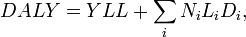
where i is an index for all diseases considered. See also the Wikipedia article about Disability-adjusted life year.

QALY

Main article: Quality-adjusted life year

Quality-adjusted life year is similar to disability-adjusted life year. The main difference is that instead of calculating cases of particular diseases, people's quality of life is evaluated using a typically five-dimensional quality indicator about e.g. functionality, pain, anxiety. See also the Wikipedia article about Quality-adjusted life year.

Number of cases

Number of cases of disease or death is a straightforward and easily understandable indicator. There are several ways of estimating it, and some of them have been described in Attributable risk. Other methods exist as well, e.g. additional cases may be estimated by comparing typical numbers of disease to the increased numbers during an epidemic.

Life expectancy

Main article: Life expectancy.

Life expectancy is a measure of the average expected lifetime given current conditions and risk factors. It is estimated by calculating survival function of all subsequent age groups. It is useful for population-level comparisons and policy discussions. However, it is a problem that estimates about absolute differences due to specific risk factor are so small that they appear meaningless even if they are important for the particular population or situation.

Welfare indicators

National sets of indicators:

Measures of Australia’s progress
Canadian Index of well-being
U.S. Key National Indicators Initiative (web-based database)
Measuring Ireland’s Progress
UK.s Quality of Life Counts

International sets of indicators:

UN: Millennium Development Goals Indicators
Eurostat: Sustainable Development Indicators
EU strategy for social protection and inclusion indicators (14)
OECD Factbook -> coming up: Handbook of Measuring Progress

Single indicators:

The Genuine Progress Indicator
Human Development Index - Human Poverty Index
The Measure of Economic Welfare
Index of Sustainable Welfare
WISP (World Index for Social Progress)
Composite Learning Index
Happy Planet Index
Measure of Domestic Progress (NEF)
Sustainable National Income (SNI)
OECD; Handbook on Constructing Composite Indicators (2005)

References

Attributable risk method

**Progression class**
In Opasnet many pages being worked on and are in different classes of progression. Thus the information on those pages should be regarded with consideration. The progression class of this page has been assessed: This page is a full draft This page has been written through once, so all important content is already where it should be. However, the content has not been thoroughly checked yet, and for example important references might still be missing.	The content and quality of this page is/was being curated by the project that produced the page.

This page is a knowledge crystal of subtype method. The page identifier is Op_en7493
Moderator:Jouni (see all)

Upload data Show results

Attributable risk is a fraction of total risk that can be attributed to a particular cause. There are a few different ways to calculate it. Population attributable fraction of an exposure agent is the fraction of disease that would disappear if the exposure to that agent would disappear in a population. Etiologic fraction is the fraction of cases that have occurred earlier than they would have occurred (if at all) without exposure. Etiologic fracion cannot typically be calculated based on risk ratio (RR) alone, but it requires knowledge about biological mechanisms.

Question

How to calculate attributable risk? What different approaches are there, and what are their differences in interpretation and use?

Answer

Risk ratio (RR)

risk among the exposed divided by the risk among the unexposed

RR = \frac{R_1}{R_0}.

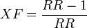
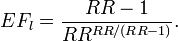
Excess fraction

(sometimes called attributable fraction) the fraction of cases among the exposed that would not have occurred if the exposure would not have taken place:

XF = \frac{RR - 1}{RR}

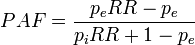
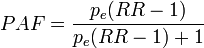
Population attributable fraction

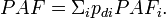
the fraction of cases among the total population that would not have occurred if the exposure would not have taken place. The most useful formulas are

PAF = 1 - \frac{1}{\sum_{i=0}^k p_i (RR_i)}

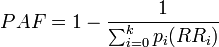
for use with several population subgroups (typically with different exposure levels). Not valid when confounding exists. Subscript i refers to the i^th subgroup. p_i = proportion of total population in i^th subgroup.

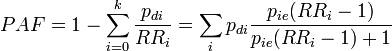
PAF = 1- \sum_{i=0}^k \frac{p_{di}}{RR_i} = \sum_i p_{di} \frac{p_{ie}(RR_i - 1)}{p_{ie}(RR_i - 1) + 1}

which produces valid estimates when confounding exists but with a problem that parameters are often not known. p_di is the proportion of cases falling in subgroup i (so that Σ_ip_di = 1), p_ie is the proportion of exposed people within subgroup i (and 1-p_ie is the fraction of unexposed)

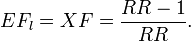
Etiologic fraction

Fraction of cases among the exposed that would have occurred later (if at all) if the exposure had not taken place. It cannot be calculated without understanding of the biological mechanism, but there are equations for several specific cases. If survival functions are known, the lower limit of EF can be calculated:

\int_G [f_1(u) - f_0(u)]\mathrm{d}u / [1 - S_1(t)],

where 1 means the exposed group, 0 means the unexposed group, f is the proportion of population dying at particular time points, S is the survival function (and thus f(u) = -dS(u)/du), t is the length of the observation time, u the observation time and G is the set of all u < t such that f₁(u) > f₀(u).

In a specific case where the survival distribution is exponential, the following formula can be used for the lowest possible EF. However, the exponential survival model says nothing about which individuals are affected and lose how much life years, and therefore in this model the actual EF may be between the lower bound and 1.

EF_l = \frac{RR - 1}{RR^{RR/(RR-1)}}.

Finally, it should be remembered that if the rank preserving assumption holds (i.e. the rank of individual deaths is not affected by exposure: everyone dies in the same order as without exposure, just sooner), the EF can be as high as 1.

EF_u = 1

With this code, you can compare excess fraction and lower (assuming exponential survival distribution) and upper bounds of etiological fraction.

+ Show code - Hide code

library(OpasnetUtils)
library(psych)
AF <- function(x) {return(data.frame(RR = x, XF = (x-1)/x, EF_exp_lower = (x-1)/x^(x/(x-1)), EF_upper = 1))}

oprint(AF(RR))

This code creates a simulated population of 200 individuals that are now 60 years of age. It calculates their survival and excess and etiologic fractions in different mechanistic settings. Relative risk of 1.2 and a constant hazard rate will be applied in all scenarios.

+ Show code - Hide code


#This is code 6211/ on page [[Attributable risk]]
library(OpasnetUtils)
library(reshape2)
library(ggplot2)

cat("Analysis of variation in etiologic fraction. Parameters:\n")
if(linear) cat("Uniform survival distribution (people die between 60 and 80 years)\n") else
  cat("Exponential survival distribution (remaining life expectancy at 60 year is 10 years\n")
if(shuffle == 1) {
  cat("Preserve rank order of individual lifetimes\n")
} else {
  if(shuffle == 2) {
    cat("Minimize EF by accumulating life loss to the hardy\n")
  } else {
    cat("Shuffle lifetimes with approximate rank correlation\n")
  }
}

#linear <- TRUE
#scenario <- c(1, 2, 3)
#crr <- NULL
RR. <- 1.2

objects.latest("Op_en6007", code_name = "answer") # Fetch correlvar

lifetime <- data.frame(
  Unexposed = if(linear) seq(0, 20, 0.1) else qexp((1:200)/201, 1/10)
)

yll <- mean(lifetime$Unexposed) * (RR. - 1) / RR.

if(1 %in% scenario) {
  lifetime$ConstantSurvShift <- lifetime$Unexposed - yll
}
#if(2 %in% scenario) {
#  sequ <- RR. / (RR. - 1)
#  temp <- round(1:(nrow(lifetime) / sequ) * sequ)
#  lifetime$AFdistribution <- lifetime$Unexposed
#  lifetime$AFdistribution[temp] <- lifetime$Unexposed[temp] - yll * sequ
#}

if(2 %in% scenario) {
  lifetime$CompetingCauses <- if(linear) {
    seq(0, by = 0.1/RR., length.out = nrow(lifetime))
  } else {
    qexp((1:200)/201, 1/10*RR.)
  }
}

cat("Individual lifetimes in the population when order is preserved.\n")
oprint(lifetime)

# Minimize EF by sorting

if(shuffle == 2) {
  for(j in colnames(lifetime)[!colnames(lifetime) %in% c("Id", "Unexposed")]) {
    for(i in 1:nrow(lifetime)) {
      pos <- match(TRUE, lifetime$Unexposed[i] <= lifetime[i:nrow(lifetime) , j]) + i - 1
      if(pos > i & !is.na(pos)) {
        block1 <- if(i < 2) numeric() else 1:(i - 1)
        block2 <- if(pos == nrow(lifetime)) numeric() else (pos+1):nrow(lifetime)
        temp <- c(block1, pos, i:(pos-1), block2)
        if(length(temp) == nrow(lifetime)) {
          lifetime[[j]] <- lifetime[temp , j]
        } else {
          warning("Vectors do not match: i ", i, ", pos ", pos, ", temp ", temp)
        }
      }
    }
  }
  cat("Individual lifetimes in the population when life loss is accumulated to the hardy.\n")
  oprint(lifetime)
}

# Shuffle individuals in different scenarios

if(shuffle == 3) {
  Sigma <- matrix(crr, nrow = ncol(lifetime), ncol = ncol(lifetime)) + diag(ncol(lifetime))*(1 - crr)
  lifetime <- correlvar(lifetime, Sigma)
  lifetime <- lifetime[order(lifetime$Unexposed) , ]

  for(j in colnames(lifetime)[colnames(lifetime) != "Unexposed"]) {
    for(i in order(lifetime[[j]], decreasing = TRUE)) {
      pos <- match(TRUE, lifetime[i,j] <= lifetime$Unexposed)
      if(pos > i & !is.na(pos)) {
        block1 <- if(i < 2) numeric() else 1:(i - 1)
        block2 <- if(pos == nrow(lifetime)) numeric() else (pos+1):nrow(lifetime)
        temp <- c(block1, (i+1):pos, i, block2)
        if(length(temp) == nrow(lifetime)) {
          lifetime[[j]] <- lifetime[temp , j]
        } else {
          warning("Vectors do not match: i ", i, ", pos ", pos, ", temp ", temp)
        }
      }
    }
  }
}

cat("Rank correlation coefficients.\n")
oprint(cor(lifetime, method = "spearman"))

plot(lifetime)

lifetime$Id <- 1:nrow(lifetime)
objects.latest("Op_en6211", code_name = "EF")

RR <- EvalOutput(RR)

cat("Relative risks observed in the model.\n")
oprint(RR@output)

lif <- lif + 60 
# Only after the RR and le have been calculated, we can start talking about the 
# total life expectancy rather than the remaining life expectancy at 60 a.

metrices <- EvalOutput(metrices)

cat("Different etiologic and attributable fractions.\n")
oprint(unkeep(metrices, sources = TRUE))

oline <- data.frame(A = c(
  min(result(lif)[lif$Scenario == "Unexposed"]),
  max(result(lif)[!lif$Scenario %in% c("Id", "Unexposed")])
))

plotting <- lif[lif$Scenario == "Unexposed" , colnames(lif@output) != "Scenario"]
plotting <- plotting + lif - lif

BS <- 24

ggplot()+geom_point(data = plotting@output, aes(x = lifResult, y = Result, colour = Scenario))+
  geom_line(data = oline, aes(x = A, y = A)) + theme_gray(base_size = BS)+
  labs(
    title = "Scatter plot of individual lifetimes",
    x = "Unexposed (years)",
    y = "Exposed (years)"
  )

ggplot(lif@output, aes(x = Id, y = lifResult, colour = Scenario))+geom_point()+
 theme_gray(base_size = BS) + labs(title = "Life expectancies of 200 individuals", y = "Age at death", x = "Individual")

ggplot(fr@output, aes(x = Time, y = frResult, colour = Scenario, group = Scenario))+
  geom_line() + 
  theme_gray(base_size = BS)+
  theme(axis.text.x = element_text(angle = 90, hjust = 1)) +
  labs(title = "fraction of people dying at different time groups")
  
ggplot(surv@output, aes(x = Time, y = survResult, colour = Scenario, group = Scenario))+geom_line() + 
 theme_gray(base_size = BS) + labs(title = "Survival curves in different scenarios")+
  theme(axis.text.x = element_text(angle = 90, hjust = 1))
  
ggplot(EF_eq9@output, aes(x = Time, y = EF_eq9Result, colour = Scenario, group = Scenario))+geom_line()+
 theme_gray(base_size = BS) + labs(title = "Development of etiologic fraction in time")+
  theme(axis.text.x = element_text(angle = 90, hjust = 1))

Rationale

Definitions of terms

There are several different kinds of proportions that sound alike but are not. Therefore, we explain the specific meaning of several terms.

Number of people (N)

The number of people in the total population considered, including cases, non-cases, exposed and unexposed. N₁ and N_o are the numbers of exposed and unexposed people in the population, respectively.

Classifications

There are three classifications, and every person in the total population belongs to exactly one group in each classification.

Disease (D): classes case (c) and non-case (nc)
Exposure (E): classes exposed (1) and unexposed (0)
Population subgroup (S): classes i = 0, 1, 2, ..., k (typically based on different exposure levels)
Confounders (C): other factors correlating with exposure and disease and thus potentially causing bias in estimates unless measured and adjusted for.

Excess fraction (XF): The proportion of exposed cases that would not have occurred without exposure on population level.
Etiologic fraction (EF): The proportion of exposed cases that would have occurred later (if at all) without exposure on individual level.
Hazard fraction (HF): The proportion of hazard rate that would not be there without exposure, HF = [h₁(t) - h₀(t)]/h₁(t) = [R(t) - 1]/R(t), where h(t) is hazard rate at time t and R(t) = h₁(t)/h₀(t).
Attributable fraction (AF): An ambiguous term that has been used for excess fraction, etiologic fraction and hazard fraction without being specific. Therefore, its use is not recommended.
Population attributable fraction (PAF): The proportion of all cases (exposed and unexposed) that would not have occurred without exposure on population level. PAF_i is PAF of subgroup i.
Risk of disease (hazard rates): R₁ and R₀ are the risks of disease in the exposed and unexposed group, respectively, and RR = R₁ / R₀. RR_i = relative risk comparing i^th exposure level with unexposed group (i = 0). Note that often texts are not clear when they talk about risk proportion = number of cases / number of population and thus risk ratio; and when about hazard rates = number of cases / observation time and thus rate ratio. RR may mean either one. If occurrence of cases is small, risk ratio and rate ratio approach each other, because then cases hardly shorten the observation time in the population.
Proportion exposed (p_e, p_ie, p_ed): proportion of exposed among the total population or within subgroup i or within cases (we use subscript d as diseased rather than c as cases to distinguish it from subscript e): p_e = N(E=1)/N, p_ie = N(E=1,S=i)/N(S=i), p_ed = N(E=1,D=c)/N(D=c)
Proportion of population (p_i): proportion of population in subgroups i among the total population: N(S=i)/N. p'_i is the fraction of population in a counterfactual ideal situation (where the exposure is typically lower).
Proportion of cases of the disease (p_di): proportion of cases in subgroups i among the total cases: N(D=c,S=i)/N(D=c) (so that Σ_ip_di = 1).

Excess fraction

Rockhill et al.^[1] give an extensive description about different ways to calculate excess fraction (XF) and population attributable fraction (PAF) and assumptions needed in each approach. Modern Epidemiology ^[2] is the authoritative source of epidemiology. They first define excess fraction XF for a cohort of people (pages 295-297). It is the fraction of cases among the exposed that would not have occurred if the exposure would not have taken place.R↻ However, both sources use the term attributable fraction rather than excess fraction.

Impact of confounders

Darrow and Steenland^[3] studied the direction and magnitude of bias in excess fraction with different confounding situations.

The problem with the two PAF equations (see Answer) is that the former has easier-to-collect input, but it is not valid if there is confounding. It is still often mistakenly used. The latter equation would produce an unbiased estimate, but the data needed is harder to collect. Darrow and Steenland^[3] have studied the impact of confounding on the bias in attributable fraction. This is their summary:

**The impact of confounding on the bias in excess fraction.**
Bias in excess fraction	Confounding in RR	Confounding in inputs
AF bias (-), calculated AF is smaller than true AF	Conf RR (+), crude RR is larger than adjusted (true) RR	Confounder is positively associated with exposure and disease (++)
AF bias (-), calculated AF is smaller than true AF	Conf RR (+), crude RR is larger than adjusted (true) RR	Confounder is negatively associated with exposure and disease (--)
AF bias (+), calculated AF is larger than true AF	Conf RR (-), crude RR is smaller than adjusted (true) RR	Confounder is negatively associated with exposure and positively with disease (-+)
AF bias (+), calculated AF is larger than true AF	Conf RR (-), crude RR is smaller than adjusted (true) RR	Confounder is positively associated with exposure and negatively with disease (+-)

Population attributable fraction

The population attributable fraction PAF is the fraction of all cases (exposed and unexposed) that would not have occurred if the exposure had been absent.

**Different ways to calculate population attributable fraction PAF.**
#	Formula	Description
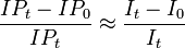
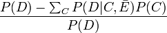
1	$\frac{IP_t - IP_0}{IP_t} \approx \frac{I_t - I_0}{I_t}$	is empirical approximation of ^[1] $\frac{P(D) - \sum_C P(D\|C, \bar{E}) P(C)}{P(D)}$ where IP₁ = cumulative proportion of total population developing disease over specified interval; IP₀ = cumulative proportion of unexposed persons who develop disease over interval, C means other confounders, and E is exposure and a bar above E means no exposure. Valid only when no confounding of exposure(s) of interest exists. If disease is rare over time interval, ratio of average incidence rates I₀/I_t approximates ratio of cumulative incidence proportions, and thus formula can be written as (I_t - I₀)I_t. Both formulations found in many widely used epidemiology textbooks. ⇤--#: . Is there an error in the text about the approximation? --Jouni (talk) 10:05, 28 June 2016 (UTC) (type: truth; paradigms: science: attack)
2	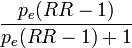$\frac{p_e(RR-1)}{p_e(RR-1)+1}$	Transformation of formula 1.^[1] Not valid when there is confounding of exposure-disease association. RR may be ratio of two cumulative incidence proportions (risk ratio), two (average) incidence rates (rate ratio), or an approximation of one of these ratios. Found in many widely used epidemiology texts, but often with no warning about invalidness when confounding exists.
3	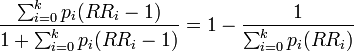$\frac{\sum_{i=0}^k p_i (RR_i - 1)}{1 + \sum_{i=0}^k p_i (RR_i - 1)} = 1 - \frac{1}{\sum_{i=0}^k p_i (RR_i)}$	Extension of formula 2 for use with multicategory exposures. Not valid when confounding exists. Subscript i refers to the i^th exposure level. Derived by Walter^[4]; given in Kleinbaum et al.^[5] but not in other widely used epidemiology texts.
4	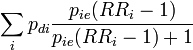$\sum_i p_{di} \frac{p_{ie}(RR_i - 1)}{p_{ie}(RR_i - 1) + 1}$	A useful formulation from^[3]. Note that RR_i is the risk ratio for subgroup i due to the subgroup-specific exposure level and assumes that everyone in that subgroup is exposed to that level or none.
5	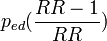$p_{ed}(\frac{RR-1}{RR})$	Alternative expression of formula 3.^[1] Produces internally valid estimate when confounding exists and when, as a result, adjusted relative risks must be used.^[6] In Kleinbaum et al.^[5] and Schlesselman.^[7]
6	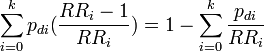$\sum_{i=0}^k p_{di} (\frac{RR_i - 1}{RR_i}) = 1- \sum_{i=0}^k \frac{p_{di}}{RR_i}$	Extension of formula 5 for use with multicategory exposures.^[1] Produces internally valid estimate when confounding exists and when, as a result, adjusted relative risks must be used. See Bruzzi et al. ^[8] and Miettinen^[6] for discussion and derivations; in Kleinbaum et al.^[5] and Schlesselman.^[7]

$PAF = \frac{N_1 (R_1 - R_0)}{N_1 R_1 + N_0 R_0} = \frac{N_1 (R_1 - R_0)/R_0}{N_1 R_1/R_0 + N_0 R_0/R_0} = \frac{N_1 (RR - 1)}{N_1 RR + N_0}$

$= \frac{ \frac{N_1 (RR - 1)}{N_1 + N_0} }{ \frac{N_1 RR + N_0}{N_1 + N_0}} = \frac{ p_e (RR - 1) }{ \frac{N_1 RR - N_1 + (N_1 + N_0)}{N_1 + N_0}} = \frac{p_e (RR - 1)}{p_e RR - p_e + 1} = \frac{p_e (RR - 1)}{p_e (RR - 1) + 1}.$

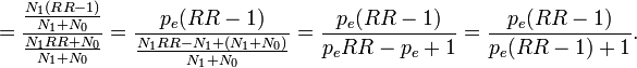
Note that there is a typo in the Modern Epidemiology book: the denominator should be p(RR-1)+1, not p(RR-1)-1.

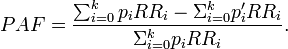
Population attributable fraction can be calculated as a weighted average based on subgroup data:

$PAF = \Sigma_i p_{di} PAF_{i}.$

Specifically, we can divide the cohort into subgroups based on exposure (in the simplest case exposed and unexposed), so we get

$PAF = p_{ed} \frac{1(RR - 1)}{1(RR - 1) + 1} + (1 - p_{ed}) \frac{0(RR - 1)}{0(RR - 1) +1} = p_{ed} \frac{RR - 1}{RR},$

where p_c is the proportion of cases in the exposed group among all cases; this is the same as exposure prevalence among cases.

WHO approach

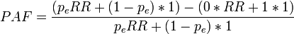
According to WHO, PAF is ^[9]

$PAF = \frac{\sum_{i=0}^k p_i RR_i - \Sigma_{i=0}^k p'_i RR_i}{\Sigma_{i=0}^k p_i RR_i}.$

We can see that this reduces to PAF equation 2 when we limit our examination to a situation where there are only two population groups, one exposed to background level (with relative risk 1) and the other exposed to a higher level (with relative risk RR). In the counterfactual situation nobody is exposed. in this specific case, p_i = p_e. Thus, we get

$PAF = \frac{(p_e RR + (1-p_e)*1) - (0*RR + 1*1)}{p_e RR + (1-p_e)*1}$

$PAF = \frac{p_e RR - p_e}{p_i RR + 1 - p_e}$

$PAF = \frac{p_e(RR - 1)}{p_e(RR -1) + 1}$

----#: . Constant background assumption section was archived because it was only relevant for a previous HIA model version. --Jouni (talk) 13:17, 25 April 2016 (UTC) (type: truth; paradigms: science: comment)

Etiologic fraction

Uniform survival means that deaths will occur at constant absolute rate between 60 and 80 years of age. In the exposed situation, the rate is higher by a factor of RR = 1.2 in this case.

Although the survival curve can be observed, we don't know which individuals would have died in a counterfactual situation. Here we assume that we know that. On the left, the order of deaths is preserved irrespective of exposure, while on the right, the maximum amount of life loss is concentrated to the minimum number of individuals, thus minimizing the etiologic fraction. Black line: one-to-one relationship between lifetimes in unexposed and exposed situations.

Etiologic fraction (EF) is defined as the fraction of cases that are advanced in time because of exposure.^[10]R↻ In other words, those cases would have occurred later (if at all), if there had not been exposure. EF can also be called probability of causation, which has importance in court. It can also be used to calculate premature cases, but that term is ambiguous and sometimes it is used to mean cases that have been substantially advanced in time, in contrast to the harvesting effect where an exposure kills people that would have died anyway within a few days. There has been a heated discussion about harvesting effect related to fine particles. Therefore, sometimes excess fraction is used instead to calculate what they call premature mortality, but unfortunately that practice causes even more confusion.R↻ Therefore, it is important to explicitly explain what is meant by the word premature.

Robins and Greenland^[10] studied the estimability of etiologic fraction. They concluded that observations are not enough to conclude about the precise value of EF, because irrespective of observation, the same amount of observed life years lost may be due to many people losing a short time each, or due to a few losing a long time each. The upper limit in theory is always 1, and the lower bound they estimated by this equation (equation 9 in the article):

$\int_G [f_1(u) - f_0(u)]\mathrm{d}u / [1 - S_1(t)],$

where 1 means the exposed group, 0 means the unexposed group, f is the proportion of population dying at particular time points, S is the survival function (and thus f(u) = -dS(u)/du), t is the length of the observation time, u the observation time and G is the set of all u < t such that f₁(u) > f₀(u).

Although the exact value of etiologic fraction cannot be estimated directly from risk ratio (RR), different models offer equations to estimate EF. It is just important to understand, discuss, and communicate, which of the models most closely represents the actual situation observed. Three models are explained here.R↻

Rank-preserving model says that everyone dies at the same rank order as without exposure, but that the deaths occur earlier. If the exposed population loses life years compared with unexposed population, it is in theory always possible that everyone dies a bit earlier and thus

$EF_u = 1.$

Competing causes model is the most commonly assumed model, but often people do not realise that they make such an assumption. The model says that the exposure of interest and other causes of death are constantly competing, and that the impact of the exposure is relative to the other competing causes. In other words, the hazard rate in the exposed population is h₁(t) = RR h₀(t). Hazard rates are functions of time, and may become very high in very old populations. In any case, the proportional impact of the exposure stays constant.

In the case where competing causes model and independence assumtption applies, lower end of EF range is often close to the excess fraction XF. (But it can be lower, as the next example with a skewed exponential distribution demonstrates.)

$EF_l = XF = \frac{RR - 1}{RR}.$

Exponential survival model assumes that the hazard rate is constant and the deaths occur following the exponential distribution. Although this model has very elegant formulas, it is typically far from plausible, as the differences in survival may be very large. E.g. with average life expectancy of 70 years, 10 % of the population would die before 8 years of age, while 10 % would live beyond 160 years. In situations where exponential survival model can be used, the lower bound of EF (equation 9^[10]) is as low as

$EF_l = \frac{RR - 1}{RR^{RR/(RR-1)}}.$

For an illustration of the behaviour of EF, see the code "Test different etiologic fractions" in the Answer. Also the true etiologic fraction is calculated for this simulated population, because in the simulation we assume that we know exactly what happens to each individual in each scenario and how much their lengths of lives change. By testing with several inputs, we can see the following pattern (table).

**Different ways to calculate etiologic and excess fractions.**
Equations 9 and 11 refer to Robins and Greenland^[10]. True EF is calculated by comparing individual lifetimes in counterfactual situations in the model. Low means the lower confidence limit.
Survival distribution	Scenario	Excess fraction XF	True etiologic fraction	EF_low from Eq 9	EF_low from Eq 11
Uniform	Competing causes, minimize EF[9]	0.17	0.17	0.17	0.07
Uniform	Competing causes, preserve rank order[10]	0.17	1.00	0.17	0.07
Exponential	Competing causes, minimize EF[11]	0.17	0.07	0.07	0.07
Exponential	Competing causes, preserve rank order[12]	0.17	1.00	0.07	0.07

As we can see from the table, true etiologic fraction can vary substantially - in theory. High values assume that most people are affected by a small life loss. This might be true with causes that worsen general health, thus killing the person a bit earlier than what would have happened if the person had been in a hardier state.

When we compare equations 9 and 11, we can see that the former never performs worse than the latter. This is simply because equation 11 was derived from equation 9 by making an additional assmuption that the survival distribution is exponential. Indeed, in such a case they produce identical values but in other cases equation 11 underestimates EF compared with equation 9. A practical conclusion is that if survival curves for exposed and unexposed groups are available, equation 9 rather than equation 11 should always be used. Even excess fraction is usually a better estimate than an estimate from equation 11, with the exception of exponential survival distribution.

Calculations

⇤--#: . UPDATE AF TO REFLECT THE CURRENT IMPLEMENTATION OF ERF Exposure-response function --Jouni (talk) 05:20, 13 June 2015 (UTC) (type: truth; paradigms: science: attack)

+ Show code - Hide code

# This is code Op_en6211/AF on page [[Attributable risk]]
# Parameters: none

library(OpasnetUtils)

# AF = attributable fraction
# EF = etiologic fraction
# PAF = population attributable fraction using 
EF <- Ovariable("EF", 
	dependencies = data.frame(Name = c(
		"RR" # Risk ratio
	)),
	
	formula = function(...) {

		R <- unkeep(RR, sources = TRUE, prevresults = TRUE)
		EF <- (RR - 1) / R^(R/(R-1))
		EF <- EF * Ovariable("temp", data = data.frame(
			EFestimate = c("Low", "High"),
			Result = 1
		))
		result(EF)[EF$EFestimate == "High"] <- 1

		return(EF)
	}
)

AF <- Ovariable("AF", 
	dependencies = data.frame(Name = c(
		"RR" # Risk ratio
	)),
	
	formula = function(...) {

		AF <- (RR - 1) / unkeep(RR, sources = TRUE, prevresults = TRUE)

		return(AF)
	}
)

PAF <- Ovariable("PAF", 
	dependencies = data.frame(Name = c(
		"RR", # Risk ratio
		"pci", # proportion of cases falling subgroup i among all cases
		"pei" # proportion of exposed people within subgroup i
	)),
	
	formula = function(...) {

		peirri <- pei * (RR - 1)
		peirri <- unkeep(peirri, sources = TRUE, prevresults = TRUE)

		PAF <- pci * peirri / (peirri + 1) # The population subgroup could be summed up.

		return(PAF)
	}
)

objects.store(EF, AF, PAF)
cat("Ovariables EF, AF, PAF stored.\n")

A previous version of code looked at RRs of all exposure agents and summed PAFs up.

Some interesting model runs:

+ Show code - Hide code

#This is code Op_en6211/EF on page [[Attributable risk]]

library(OpasnetUtils)

lif <- Ovariable(
  "lif",
  dependencies = data.frame(Name = "lifetime"),
  formula = function(...) {
    out <- melt(
       lifetime, 
       id.vars = "Id", 
       value.name = "Result", 
       variable.name = "Scenario"
    )
    out <- Ovariable(
      output = out, 
      marginal = c(TRUE, TRUE, FALSE)
    )
    return(out)
  }
)

le <- Ovariable(
  "le",
  dependencies = data.frame(Name = "lif"),
  formula = function(...) {
    le <- oapply(lif, INDEX = "Scenario", FUN = sum) / 
    oapply(lif, INDEX = "Scenario", FUN = length)
    return(le)
  }
)

RR <- Ovariable(
  "RR",
  dependencies = data.frame(Name = "le"),
  formula = function(...) {
    RR <- le[le$Scenario == "Unexposed" , ]
    RR <- unkeep(RR, cols = c("Scenario", "lifResult"))
    RR <- RR / le
    RR <- unkeep(RR, prevresults = TRUE)
    return(RR)
  }
)

fr <- Ovariable("fr", 
  dependencies = data.frame(
    Name = "lif"
  ),
  formula = function(...) {
    out <- lif
    temp2 <- cut(result(out), breaks = 12)
    out$Time <- temp2
    out <- out * 0 + 1/oapply(out, cols = c("Id", "Time"), FUN = length)
    temp <- Ovariable(
      "temp", 
      data = data.frame(
        Time = levels(temp2),
        Result = 0
      )
    )
    out <- combine(EvalOutput(temp), out)
    out <- oapply(out, cols = "Id", FUN = sum) # Automatic fillna is OK.
    return(out)
  }
)

surv <- Ovariable(
  "surv",
  dependencies = data.frame(Name = "fr"),
  formula = function(...) {
    out <- fr[order(fr$Time) , ]
    temp <- data.frame()
    for(i in unique(out$Scenario)) {
      temp2 <- out[out$Scenario == i , ]
      result(temp2) <- 1 - cumsum(result(temp2))
      temp <- rbind(temp, temp2@output)
    }
    out@output <- temp
    return(out)
  }
)

EF_eq9 <- Ovariable(
  "EF_eq9",
  dependencies = data.frame(Name = c("fr", "surv")),
  formula = function(...) {
    BAU <- fr[fr$Scenario == "Unexposed" , ]
    BAU <- unkeep(BAU, prevresults = TRUE, sources = TRUE, cols = "Scenario")
    
    out <- fr
    result(out) <- pmax(0, result(out - BAU))
    
    out <- out[order(out$Time) , ]
    temp <- data.frame()
    for(i in unique(out$Scenario)) {
      temp2 <- out[out$Scenario == i , ]
      result(temp2) <- cumsum(result(temp2))
      temp <- rbind(temp, temp2@output)
    }
    out@output <- temp
    out <- out / (1 - surv)
    
    return(out)
  }
)

EF_true <- Ovariable(
  "EF_true", 
  dependencies = data.frame(Name = "lif"),
  formula = function(...) {
    BAU <- lif[lif$Scenario == "Unexposed" , ]
    BAU <- unkeep(BAU, cols = "Scenario", prevresults = TRUE, sources = TRUE)
    out <- lif < BAU
    out <- oapply(out, cols = "Id", FUN = sum) / 
      oapply(out, cols = "Id", FUN = length)
    
    return(out)
  }
)

metrices <- Ovariable(
  "metrices", 
  dependencies = data.frame(Name = c("RR", "lif", "EF_true", "EF_eq9")),
  formula = function(...) {
    out <- (RR - 1) / RR
    out$Metric <- "Attributable fraction"
    temp <- (RR - 1)/(RR^(RR/(RR-1)))
    temp$Metric <- "EF_low from eq 11"
    out <- combine(out, temp)
#    result(temp) <- 1
#    temp$Metric <- "EF_up theoretical"
#    out <- combine(out, temp)
    temp <- unkeep(EF_true, sources = TRUE, prevresults = TRUE)
    temp$Metric <- "EF_true"
    out <- combine(out, temp)
    temp <- unkeep(EF_eq9[EF_eq9$Time == levels(EF_eq9$Time)[length(levels(EF_eq9$Time))] , ],
           cols = "Time", sources = TRUE, prevresults = TRUE
    )
    temp$Metric <- "EF_low from Eq 9"
    out <- combine(out, temp)
    

    return(out)
  }
)

objects.store(lif, le, RR, fr, surv, EF_eq9, EF_true, metrices)
cat("Ovariables lif, le, RR, fr, surv, EF_eq9, EF_true, metrices stored.\n")

Demonstration of hazard fractions, survival, and age at death

Figure for manuscript Morfeld, Erren, Hammit etc.

+ Show code - Hide code

library(ggplot2)
library(reshape2)

# Data from https://www.ssa.gov/oact/STATS/table4c6.html

h1 <- c( # Probability of dying per year by age (0-119 years)
	0.006322,
	0.000396,
	0.000282,
	0.000212,
	0.000186,
	0.000162,
	0.000144,
	0.000129,
	0.000114,
	0.0001,
	0.000093,
	0.000101,
	0.000136,
	0.000205,
	0.000299,
	0.000401,
	0.000505,
	0.00062,
	0.000747,
	0.000879,
	0.001019,
	0.001151,
	0.001252,
	0.001309,
	0.001335,
	0.001349,
	0.001369,
	0.001391,
	0.001422,
	0.001459,
	0.001498,
	0.001536,
	0.001576,
	0.001616,
	0.001661,
	0.001716,
	0.001782,
	0.001854,
	0.001931,
	0.002018,
	0.002123,
	0.002252,
	0.002413,
	0.002611,
	0.002845,
	0.003109,
	0.003402,
	0.003736,
	0.004114,
	0.004533,
	0.004987,
	0.005473,
	0.005997,
	0.00656,
	0.007159,
	0.007803,
	0.00848,
	0.00917,
	0.009863,
	0.010572,
	0.011354,
	0.012202,
	0.013061,
	0.01392,
	0.014819,
	0.015826,
	0.016986,
	0.018295,
	0.019776,
	0.021448,
	0.02338,
	0.025549,
	0.027885,
	0.030374,
	0.033099,
	0.036254,
	0.039882,
	0.043879,
	0.048256,
	0.053123,
	0.058711,
	0.065081,
	0.072139,
	0.079912,
	0.088529,
	0.098148,
	0.108902,
	0.120886,
	0.134149,
	0.148699,
	0.164525,
	0.1816,
	0.199884,
	0.219331,
	0.239886,
	0.260269,
	0.280109,
	0.299013,
	0.316578,
	0.332406,
	0.349027,
	0.366478,
	0.384802,
	0.404042,
	0.424244,
	0.445456,
	0.467729,
	0.491116,
	0.515671,
	0.541455,
	0.568528,
	0.596954,
	0.626802,
	0.658142,
	0.691049,
	0.725602,
	0.761882,
	0.799976,
	0.839975,
	0.881973
)
h0 <- h1/1.5
df <- data.frame(
	Age = 0:119,
	h1 = h1,
	h0 = h0,
	S1 = exp(-cumsum(h1)),
	S0 = exp(-cumsum(h0))
)
df$f1 <- df$h1 * df$S1
df$f0 <- df$h0 * df$S0
dfm <- melt(df, id.var="Age")
dfm$Exposure <- ifelse(as.numeric(substr(dfm$variable,2,2)), "Exposed","Nonexposed")
dfm$Parameter <- substr(dfm$variable,1,1)
dfm$Parameter <- factor(
	dfm$Parameter, 
	levels=c("h","S", "f"), 
	labels=c("Hazard rate h (P/year)","Survival S (P)","Age at death f (pd)")
)

pdf("//cesium/jtue$/_Documents/Survivalfunctions.pdf", height=14,width=10.5)
ggplot(dfm, aes(x=Age, y=value, linetype=Exposure))+geom_line(size=1)+
	facet_grid(Parameter~., scales="free_y")+
	labs(y="Probability (P) or probability density (pd)")+
	theme_bw(base_size=24)+theme(legend.position="bottom")
dev.off()

References

↑ ^1.0 ^1.1 ^1.2 ^1.3 ^1.4 Rockhill B, Newman B, Weinberg C. use and misuse of population attributable fractions. American Journal of Public Health 1998: 88 (1) 15-19.[1]
↑ Kenneth J. Rothman, Sander Greenland, Timothy L. Lash: Modern Epidemiology. Lippincott Williams & Wilkins, 2008. 758 pages.
↑ ^3.0 ^3.1 ^3.2 Darrow LA, Steenland NK. Confounding and bias in the attributable fraction. Epidemiology 2011: 22 (1): 53-58. [2] doi:10.1097/EDE.0b013e3181fce49b
↑ Walter SD. The estimation and interpretation of attributable fraction in health research. Biometrics. 1976;32:829-849.
↑ ^5.0 ^5.1 ^5.2 Kleinbaum DG, Kupper LL, Morgenstem H. Epidemiologic Research. Belmont, Calif: Lifetime Learning Publications; 1982:163.
↑ ^6.0 ^6.1 Miettinen 0. Proportion of disease caused or prevented by a given exposure, trait, or intervention. Am JEpidemiol. 1974;99:325-332.
↑ ^7.0 ^7.1 Schlesselman JJ. Case-Control Studies: Design, Conduct, Analysis. New York, NY: Oxford University Press Inc; 1982.
↑ Bruzzi P, Green SB, Byar DP, Brinton LA, Schairer C. Estimating the population attributable risk for multiple risk factors using case-control data. Am J Epidemiol. 1985; 122: 904-914.
↑ WHO: Health statistics and health information systems. [3]. Accessed 16 Nov 2013.
↑ ^10.0 ^10.1 ^10.2 ^10.3 Robins JM, Greenland S. Estimability and estimation of excess and etiologic fractions. Statistics in Medicine 1989 (8) 845-859.

Discussion about attributable risk method

Note! There are several references to Verses on this page. All the original verses are not here but on the original page heande:Talk:Population attributable fraction (password required).

Scientific disputes possibly related to attributable risk

Arch Toxicol 2009

Slama et al (2007) Environ Health Perspect 115(9):1283-1292.
Morfeld P (2009) Arch Toxicol 83:105-106.
Slama et al (2009) Arch Toxicol 83:293-295.
A plea for rigorous and honest science: false positive findings and biased presentations in epidemiological studies - Springer.[14],accessed 2016-05-12.
Comment on Slama R, Cyrys J, Herbarth O, Wichmann H-E, Heinrich J. (2009) A further plea for rigorous science and explicit disclosure of potential conflicts of interest. Morfeld P. (2009) A plea for rigorous and honest science—false positive findings and biased presentations in epidemiological studies. Archives of Toxicology 83:105–106 - Springer.[15],accessed 2016-05-12.
Comment on Slama R, Cyrys J, Herbarth O, Wichmann H-E, Heinrich J. saying: “The authors did not wish to reply, given Dr. Morfeld’s persistence in refusing to fill in the conflict of interest statement and in misleadingly quoting parts of the sentences of our publications” - Springer.[16],accessed 2016-05-12.
⇤--#: . A dispute about choosing new endpoints based on non-significance of analyses planned a priori. Not relevant discussion for attributable risk. --Jouni (talk) 13:13, 13 May 2016 (UTC) (type: truth; paradigms: science: attack)

Inhalation Toxicology 2013

(2013-01-01) "Reply to the “Letter to the Editor” by Morfeld et al.". Inhalation Toxicology 25 (1): 65–65. doi:10.3109/08958378.2012.753492. ISSN 0895-8378. Retrieved on 2016-05-12.
⇤--#: . Dispute about microscopical slicing techniques of nanoparticles. Not relevant discussion for attributable risk. --Jouni (talk) 13:13, 13 May 2016 (UTC) (type: truth; paradigms: science: attack)

Arch Toxicol 2013

Commentary to Gebel 2012: a quantitative review should apply meta-analytical methods - Springer.[17],accessed 2016-05-12.
⇤--#: . A dispute about meta-analytic methods. Not relevant discussion for attributable risk. --Jouni (talk) 13:13, 13 May 2016 (UTC) (type: truth; paradigms: science: attack)

J Occup Environ Med 2015

Morfeld, Peter (2015-02). "Buchanich et al (2014): The ecologic fallacy may have severely biased the findings". Journal of Occupational and Environmental Medicine / American College of Occupational and Environmental Medicine 57 (2): –13. doi:10.1097/JOM.0000000000000381. ISSN 1536-5948. PMID 25654527.
(2015-02) "Response to Morfeld:". Journal of Occupational and Environmental Medicine 57 (2): –13-e14. doi:10.1097/JOM.0000000000000397. ISSN 1076-2752. Retrieved on 2016-05-12.
⇤--#: . A dispute about interpreting the possibility of ecologic fallacy. Not relevant discussion for attributable risk. --Jouni (talk) 13:13, 13 May 2016 (UTC) (type: truth; paradigms: science: attack)

J Occup Environ Med 2016

Dell LD et al (2015) J Occup Environ Med. 57;984-997.
Morfeld P
(2016-01) "Authors' Response to Dr. Morfeld". Journal of Occupational and Environmental Medicine / American College of Occupational and Environmental Medicine 58 (1): –23. doi:10.1097/JOM.0000000000000618. ISSN 1536-5948. PMID 26716858.
⇤--#: . Dispute about multiple testing and consequent false positives. Not relevant discussion for attributable risk. --Jouni (talk) 13:13, 13 May 2016 (UTC) (type: truth; paradigms: science: attack)

Particle and Fiber Toxicology 2016

Hartwig A (2014) MAK Value Documentation 2012, 2014.
Morfeld et al (2015) Part Fibre Toxicol 12(1):3.
Hartwig a (Part Fibre Toxicol 2015
(2016-01-08) "Response to the Reply on behalf of the ‘Permanent Senate Commission for the Investigation of Health Hazards of Chemical Compounds in the Work Area’ (MAK Commission) by Andrea Hartwig Karlsruhe Institute of Technology (KIT)". Particle and Fibre Toxicology 13. doi:10.1186/s12989-015-0112-6. ISSN 1743-8977. PMID 26746196. Retrieved on 2016-05-12.
⇤--#: . A dispute about extrapolating particle deposition from rats to humans. Not relevant for attributable fraction. --Jouni (talk) 13:13, 13 May 2016 (UTC) (type: truth; paradigms: science: attack)

Int Arch Occup Environ Health 2016

Möhner M (2015) Int Arch Occup Environ Health.
Morfeld P (2015) Int Arch Occup Environ Health.
Möhner, Matthias (2016-02-22). "Response to the letter to the editor from Morfeld". International Archives of Occupational and Environmental Health: 1–2. doi:10.1007/s00420-016-1121-y. ISSN 1432-1246 0340-0131, 1432-1246. Retrieved on 2016-05-12.
----#: . Dispute about biases estimating SMR. May be relevant for attributable risk. The original paper and Morfeld's comment should be studied. --Jouni (talk) 13:13, 13 May 2016 (UTC) (type: truth; paradigms: science: comment)

Int J Public Health 2016

Morfeld, Peter (2016-04-26). "Quantifying the health impacts of ambient air pollutants: methodological errors must be avoided". International Journal of Public Health. doi:10.1007/s00038-015-0766-8. ISSN 1661-8564. PMID 27117686.
Héroux et al. Response to “Quantifying the health impacts of ambient air pollutants: methodological errors must be avoided”. International Journal of Public Health, pp 1-2.First online: 26 April 2016 doi:10.1007/s00038-016-0808-x [18]
←--#: . This is clearly relevant. Morfeld argues that excess cases do not equal premature cases. "Lim and colleagues (Lim et al 2012) relied exclusively on excess case statistics which do not allow to 'calculate the proportion of deaths or disease burden caused by specific risk factors'. Calculations of years of life lost due to exposure potientially suffer from similar problems (Morfeld 2004)." --Jouni (talk) 13:13, 13 May 2016 (UTC) (type: truth; paradigms: science: defence)

Response to Morfeld and Erren Int J Public Health

Marie-Eve Héroux, Bert Brunekreef, H. Ross Anderson, Richard Atkinson, Aaron Cohen, Francesco Forastiere, Fintan Hurley, Klea Katsouyanni, Daniel Krewski, Michal Krzyzanowski, Nino Künzli, Inga Mills, Xavier Querol, Bart Ostro, Heather Walton. Response to “Quantifying the health impacts of ambient air pollutants: methodological errors must be avoided”. International Journal of Public Health, pp 1-2.First online: 26 April 2016 doi:10.1007/s00038-016-0808-x [19]

Letter to the Editor

Response to “Quantifying the health impacts of ambient air pollutants: methodological errors must be avoided”

We thank Morfeld and Erren for their interest in our recent publication on “Quantifying the health impacts of ambient air pollutants: recommendations of a WHO/Europe project” (Héroux et al. 2015). Morfeld and Erren claim that there are potential problems with the statistical approach used in our paper to measure the impact on mortality from air pollution. In fact, they state that “Greenland showed that a calculation based on RR estimates, as performed in the EU research project, does estimate excess cases numbers—but it does not estimate the number of premature cases or etiological cases” (Greenland 1999).

Close reading of the Greenland (1999) paper reveals that he distinguishes three categories of cases occurring in the exposed, observed over a certain period of time: A0, cases which would have occurred anyway even in the absence of exposure—these would typically be estimated from the number of cases occurring in an unexposed control population; A1, cases that would have occurred anyway but were accelerated by exposure; and A2, cases which would not have occurred, ever, without exposure. The word ‘premature’ does not exist in Greenland’s paper, but we consider ‘premature’ and ‘accelerated’ to be the same here. What we usually call the attributable fraction among the exposed is equivalent to the attributable risk (RR−1)/RR which in Greenland’s paper is denoted as the etiologic fraction, (A1 + A2)/(A0 + A1 + A2). And then, etiologic cases are A1 + A2, and excess cases are A2. So, contrary to what Morfield and Erren write, the calculation as performed in our paper estimates etiologic cases (if we follow Greenland’s notation) and not excess cases. After all, in our epidemiology we cannot easily distinguish the excess cases from the accelerated cases.

But let us now take this one step further. Really, the distinction between excess cases and accelerated cases only makes sense for morbidity endpoints or for cause-specific mortality. One can envisage that some of the smokers who developed heart disease over some period of time would have developed it anyway, even in the absence of smoking, after the period of observation. We can only estimate this number A1 when we have observations of heart disease incidence in controls over a more extended period of time. Similarly, some of the smokers dying from heart disease during the period of observation might have died from heart disease anyway, but after a longer period of time. Note that the excess deaths due to heart disease A2, which would never have occurred in the smokers if they had not smoked, necessarily need to be compensated among the controls by an increase in deaths due to some other cause, as in the end, everyone dies. But for total mortality—which is where the bulk of our project’s burden estimates are based on—there are no excess cases (everybody dies in the end); so the estimates based on RR actually correctly estimate the ‘accelerated’ = ‘premature’ cases because the etiologic cases are now equivalent to the accelerated cases, in the absence of excess cases.

Interestingly, this was already described by Greenland in his example of total mortality among the A bomb survivors: “One might object that the extreme structure just described is unrealistic. In reality, however, this extremity is exactly what one should expect if the outcome under study is total mortality in a cohort followed for its entire lifetime, such as the cohort of atomic bomb survivors in Japan. Here, everyone experiences the outcome (death), so there are no “all-or-none” cases, yet everyone may also experience damage and consequent loss of years of life (even if only minor and stress related) owing to the exposure.”

This is exactly the point made by Brunekreef et al. (2007) and we note that this paper was literally and favorably quoted in a paper mentioned in support of the letter (Erren and Morfeld 2011).

The final point to stress here is that the RRs for total mortality and air pollution in our project were all derived from cohort studies in which the denominator for the number of observed cases is not the number of persons exposed or unexposed, but the person years of observation. This is, of course, for the precise reason mentioned by Greenland: if one follows a cohort until extinction, the proportion of deaths is 1 in the exposed and the unexposed alike. The RRs used in our project therefore essentially estimate the ratio of life expectancies in exposed vs. unexposed over the observation period, as the period of observation is censored at time of death and thus shorter among the exposed (who die sooner) than among the unexposed. When applied to a life table, as some of us have shown already many years ago (Brunekreef 1997; Miller and Hurley 2003), one estimates years of life lost, a major component of the Disability-Adjusted Life Years or DALYs which form the core of the GBD analyses which Morfield and Erren also disqualify as an ‘error’. As is well known, the GBD estimates are also expressed as numbers of deaths attributed to certain risk factors, and these are typically denoted as ‘premature’ deaths precisely because there is no such thing as avoidable or excess deaths when it comes to total mortality.

Therefore, in contrast to Morfeld and Erren’s assertion, our project recommendations do properly take into account methodological considerations with respect to quantification of mortality impacts of air pollution.

References

Brunekreef B (1997) Air pollution and life expectancy: is there a relation? Occup Environ Med 54:781–784. doi:10.1136/oem.54.11.781
Brunekreef B, Miller BG, Hurley JF (2007) The brave new world of lives sacrificed and saved, deaths attributed and avoided. Epidemiology 18(6):785–788
Erren TC, Morfeld P (2011) Attributing the burden of cancer at work: three areas of concern when examining the example of shift-work. Epidemiol Perspect Innov 8:4. [20]
Greenland S (1999) Relation of probability of causation to relative risk and doubling dose: a methodologic error that has become a social problem. Am J Public Health 89:1166–1169
Héroux ME et al (2015) Quantifying the health impacts of ambient air pollutants: recommendations of a WHO/Europe project. Int J Public Health 60:619–6272 doi:10.1007/s00038-015-0690-y [21]
Miller B, Hurley JF (2003) Life table methods for quantitative impact assessments in chronic mortality. J Epidemiol Community Health 57:200–206. doi:10.1136/jech.57.3.200

Copyright information © The Author(s) 2016

This is an open access article distributed under the terms of the Creative Commons Attribution IGO License ([22]), which permits unrestricted use, distribution, and reproduction in any medium, provided the original work is properly cited. In any reproduction of this article there should not be any suggestion that WHO or this article endorse any specific organization or products. The use of the WHO logo is not permitted. This notice should be preserved along with the article’s original URL.

Greenland 1999

Greenland S. Relation of probability of causation to rellative risk and doubling dose: a methologic error that has become a social problem. Am J Public Health 1999 (89) 8: 1166-69.

"When an effect of exposure is to accelerate the time at which disease occurs, the rate fraction RF = (IR - 1)/IR will tend to understate the probability of causation because it does not fully account for the acceleration of disease occurrence. In particular, and contrary to common perceptions, a rate fraction of 50% (or, equivalently, a rate ratio of 2) does not correspond to a 50% probability of causation. This discrepancy between the rate fraction and the probability of causation has been overlooked by various experts in the legal as well as the scientific community, even though it undermines the rationale for a number of current legal standards. Furthermore, we should expect this discrepancy to vary with background risk factors, so that any global assessment of the discrepancy cannot provide assurances about the discrepancies within subgroups."

----#: . Interestingly, Greenland is worried that probability of causation is underestimated when using rate fraction. --Jouni (talk) 08:34, 13 May 2016 (UTC) (type: truth; paradigms: science: comment)

Choosing the right fraction

How to read discussions

Fact discussion: .

Opening statement: Excess fraction should be used in assessing a disease fraction caused by air pollution. It is calculated with the formula XF = (RR-1)/RR, where RR is the risk ratio (risk with exposure divided by risk without exposure). The alternative is to calculate etiologic fraction EF. It cannot be estimated directly from RR, but it is always between (RR-1)/[RR^RR/(RR-1)] and 1.

Closing statement:

Excess fraction should be used to calculate health impacts when the interest is on population impact in two counterfactual exposure situations.

In contrast, etiologic fraction should be used when the interest is either probability of causation (in e.g. legal cases) or fraction of cases advanced in time due to exposure (i.e., premature cases).

(Resolved, i.e., a closing statement has been found and updated to the main page.)

Argumentation:

⇤--#1: . Excess fraction cannot be used to estimate probability of causation or fraction of cases advanced in time due to exposure (i.e., premature cases). --Jouni (talk) 14:45, 23 March 2016 (UTC) (type: truth; paradigms: science: attack)

←--#2: . By using excess fraction to estimate the number of premature deaths attributable to air pollution it is implicitly assumed that the ‘etiologic fraction’ is identical to the ‘excess fraction’.V1 --Heta (talk) 12:31, 16 March 2016 (UTC) (type: truth; paradigms: science: defence)

←--#3: . Etiologic fraction should be used instead. --Heta (talk) 12:31, 16 March 2016 (UTC) (type: truth; paradigms: science: defence)

←--#4: . In the absence of a biological model of the disease process, although the exact value of the etiologic fraction cannot be computed, bounds on the number of premature deaths attributable to exposure can be determined.V3 --Heta (talk) 12:31, 16 March 2016 (UTC) (type: truth; paradigms: science: defence)

----#5: . Estimation of the etiologic fraction is fraught with difficulty. Typically it cannot be identified without invoking strong biological assumptions.V2 --Heta (talk) 12:31, 16 March 2016 (UTC) (type: truth; paradigms: science: comment)

←--#6: . Robins and Greenland (1989) proposed replacing (RR-1)/RR by a factor f, and proved that f is bounded by (RR-1)/[RR^RR/(RR-1)] and 1. V4 --Heta (talk) 12:31, 16 March 2016 (UTC) (type: truth; paradigms: science: defence)

----#7: . At the levels of RR typical of ambient air pollution the largest possible upward bias in an estimate of the etiologic fraction derived using the excess fraction equation in lieu of f would be a factor of between 2 and 2.5.V5 --Heta (talk) 12:31, 16 March 2016 (UTC) (type: truth; paradigms: science: comment)

←--#8: . Excess fraction can be used to estimate population impact (burden of disease) in two counterfactual exposure situations. --Jouni (talk) 14:45, 23 March 2016 (UTC) (type: truth; paradigms: science: defence)

⇤--#9: . The validity of the estimates of excess deaths developed using formula (1) may be compromised by the use of RR values which have been adjusted for confounders through the use of Cox proportional hazards models.V8 --Heta (talk) 12:31, 16 March 2016 (UTC) (type: truth; paradigms: science: attack)

----#10: . Does this mean that RR values should NOT have adjusted? This needs more scrutiny. --Jouni (talk) 07:00, 24 March 2016 (UTC) (type: truth; paradigms: science: comment)

⇤--#11: . Anything in science may be wrong and compromised. Therefore, more specific argument must be provided why this particular approach is more likely to be compromised. --Jouni (talk) 07:00, 24 March 2016 (UTC) (type: truth; paradigms: science: attack)

----#12: . Excess fraction is rejected unless this fairly weak attack is accepted. --Jouni (talk) 14:45, 23 March 2016 (UTC) (type: truth; paradigms: science: comment)

←--#13: . The excess fraction can be estimated using the formula without invoking strong biological assumptions.V6 --Heta (talk) 12:31, 16 March 2016 (UTC) (type: truth; paradigms: science: defence)

----#14: . Is this the same as attributable fraction? --Heta (talk) 12:31, 16 March 2016 (UTC) (type: truth; paradigms: science: comment)

⇤--#15: . All members of a closed sub-cohort being 70 years old in 2010 (birth cohort, all born in 1940) will have died until 2050, even if all air pollution exposures would have been eliminated. Thus, the percentage of deaths until 2050 is 100% in this birth cohort even if there were no air pollution. According to formula (1), however, excess deaths will occur in this sub-cohort if exposed to air pollution in every year between 2010 and 2050. It follows that more people will die in the exposed birth cohort according to formula (1) between 2010 and 2050 than have ever lived in 2010. V12 --Heta (talk) 12:26, 17 March 2016 (UTC) (type: truth; paradigms: science: attack)

⇤--#16: . This argument is true, but potentially misleading. This paradoxical result would only occur if the approach was applied to calculate “excess deaths” in each year between 2010 and 2050 without properly adjusting the age distribution to reflect the reduced mortality at younger ages expected to flow from improvements in air quality. V14,V15 --Heta (talk) 12:26, 17 March 2016 (UTC) (type: truth; paradigms: science: attack)

----#17: . If the results in Lelieveld et al. 2015 had been characterized as ‘excess deaths’ instead of as ‘premature deaths attributable to air pollution’ much of the confusion that led to concern about our use of the formula could have been avoided.V7 --Heta (talk) 12:40, 16 March 2016 (UTC) (type: truth; paradigms: science: comment)

⇤--#18: . It would be preferable to report the results using an outcome measure, such as change in life expectancy, which explicitly reflects the impact of pollution on the timing of death.V9 --Heta (talk) 12:54, 16 March 2016 (UTC) (type: truth; paradigms: science: attack)

⇤--#19: . Which health indicator to choose is a related issue but not relevant in this argumentation, where the number of cases related to exposure has already been chosen as the indicator. --Jouni (talk) 14:45, 23 March 2016 (UTC) (type: truth; paradigms: science: attack)

⇤--#20: . Simple outcome measures, like ‘excess deaths,’ are commonly used in environmental policy analysis – where the societal benefits of various policies are estimated as the product of the value of statistical life and the number of ‘lives saved (NAS, 2002).’V11 --Heta (talk) 12:54, 16 March 2016 (UTC) (type: truth; paradigms: science: attack)

←--#21: . By doing so it might have avoided, to a large extent, the issues inherent in the interpretation of ‘premature deaths attributable to air pollution.’V10 --Heta (talk) 12:54, 16 March 2016 (UTC) (type: truth; paradigms: science: defence)

←--#22: . Effect measures which recognize the inevitability of death, such as “reduction in life expectancy” or “disability adjusted life years lost,” are clearly more readily interpretable. V13 --Heta (talk) 12:26, 17 March 2016 (UTC) (type: truth; paradigms: science: defence)

----#23: . For many purposes, measures such as "years of life lost“, "quality- (or disability-) adjusted years of life lost" are preferable.V16 --Heta (talk) 12:26, 17 March 2016 (UTC) (type: truth; paradigms: science: comment)

Meaning of premature

How to read discussions

Fact discussion: .

Opening statement: Premature mortality is about any death that is advanced in time because of a particular exposure. Similarly, premature case is a case that would occur later or not at all if there was no exposure.

Closing statement: There are different schools here and there can be two different interpretations. The first is according to the statement. The second says that a death must be advanced substantially to be denoted as premature.

(Resolved, i.e., a closing statement has been found and updated to the main page.)

Argumentation:

←--#: . This concept is important in e.g. the court, and therefore it must have a clear name. Premature is a good descriptive term for that. --Jouni (talk) 07:59, 8 April 2016 (UTC) (type: truth; paradigms: science: defence)

⇤--#: . Premature mortality should be used only about deaths that are advanced in time substantially. A few day's difference is not important. --Jouni (talk) 07:59, 8 April 2016 (UTC) (type: truth; paradigms: science: attack)

⇤--#: . Premature deaths is already widely used about all premature deaths, and people using the word for one meaning cannot prevent the usage for another meaning. --Jouni (talk) 07:59, 8 April 2016 (UTC) (type: truth; paradigms: science: attack)

⇤--#: . It should be noted that in e.g. air pollution literature, premature death means a substantial advancement of death. Air pollutants may cause deaths in terminal patients that would have died anyway within a few days. So there are at least two different interpretations. --Jouni (talk) 07:59, 8 April 2016 (UTC) (type: truth; paradigms: science: attack)

Abstract to ISEE, Rome 2016

Discussion rules as a method to resolve scientific disputes

Jouni T. Tuomisto, John S. Evans, Arja Asikainen, Pauli Ordén

Introduction: In the science-policy interface, we need better tools to synthesise discussions. We tested whether freely expressed discussions can be synthesised into resolutions using a few simple rules. We aimed at understanding key issues, not at mutual agreement of participants.

Methods: We studied two case studies about controversial topics and reorganised the information produced by participants. The topic was defined as research questions, and all content was evaluated against capability to answer the questions. The content was summarised into statments and, if possible, organised hierarchically so that statements attacked or defended one another. Statements not backed up by data were given little weight.

Results: The first case was a scientific dispute about how to estimate attributable deaths of air pollution in Lelieveld et al., Nature 2015: 525(7569):367-71. Discussion between the authors and critics was reorganised to identify and clarify the essence of the dispute. The information structure produced by the rules showed that the main dispute was about whether excess fraction or etiologic fraction should have been used. In the second case, we reorganised open web discussion about security risks caused by irregular immigrants in Finland in 2015. The discussion was held on a website coinciding with a national TV discussion. Most participants talked about their personal experience, but a few provided links to scientific studies and statistics, providing material for evidence-based discussion almost real-time.

Conclusions: Disputes about even heated and controversial topics can be clarified, understood or even resolved by using a set of rules for participation and information synthesis. Complex topics, openness, or large number of lay people participation did not hamper the process. Such rules should be tested in resolving scientific disputes on a large scale. If successful, the use of science in the society could benefit from practices of open collaboration.

Structured discussion on attributable risk of air pollution
Primary topic: Health impact assessment and participatory epidemiology
Secondary topic: Policy and public health
Presentation type: Oral or poster, no preference
Do the findings in this presentation, when combined with previous evidence, support new policy?
- Yes. Open collaboration and structured discussions could be used in resolving scientific disputes and improving the use of scientific information in the society.
No financial conflicts of interest to declare
All funding and employment resources:
- Tuomisto JT, Asikainen A were employed full time by National Institute for Health and Welfare (THL). They and Ordén P were also funded by VN-TEAS-funded project Yhtäköyttä from the Prime Minister's Office, Finland.
- Evans JS was funded by Harvard School of Public Health and Cyprus University of Technology.

Travel report

Kokous: International Society for Environmental Epidemiologists ISEE-2016
Aika: 31.8. - 5.9.2016
Paikka: Rooma, Italia
Oma esitys: Jouni T. Tuomisto, John S. Evans, Arja Asikainen, Pauli Ordén: Discussion rules as a method to resolve scientific disuputes: Case attributable risk of air pollution. (Posteri)

Vuosittainen ISEE-kokous oli tällä kertaa Roomassa Francesco Forastierin ja kumppanien järjestämänä. Osallistujia oli tavallista enemmän, käsittääkseni yli 1200. Varsinkin italialaisia oli paljon sekä järjestämässä että osallistumassa.

Kokouksen ohjelma oli perinteiseen tapaan laadukas ja monipuolinen. Erityisesti pienhiukkaset ja ilmansaasteet ylipäänsä olivat isossa roolissa. Kiinnostavaa oli myös, että etiikkatyöryhmä oli monessa sessiossa valmistellut omat puheenvuoronsa aiheen eettisistä näkökulmista, ja nämä esitykset oli numeroitu ohjelmaan erikseen. Hyvä ajatus.

Muutenkin kokouksessa näkyi vahvana epidemiologien halu tehdä vaikutus maailmaan ja parantaa kansanterveyttä (piirre jota en aikanaan toksikologien joukossa paljon huomannut). Tämä huipentui palkintojenjakogaalassa, kun Philippe Grandjean sai tunnustuspalkinnon (John Goldsmith Award for Outstanding Contributions to Environmental Epidemiology) ja puheessaan lennokkaasti korosti, että meidän on taisteltava rohkeasti ihmisten terveyden puolesta. "He eivät ole tilastolukuja vaan todellisia, kärsiviä ihmisiä." Yleisö osoitti puheelle suosiota seisaaltaan.

Oma posterini ei ollut yleisömenestys, mutta kävin kiinnostavat keskustelut mm. Heather Waltonin (UK) ja Katie Walkerin (Health Effects Institute, USA) kanssa. Heidän kanssaan kannattaa jatkaa keskustelua terveysvaikutusten arvioinnista.

Posterialueet olivat niin ahtaat, että jopa liikkuminen oli vaikeaa. Tämä kuulemma johtui siitä, että yleisömenestyksen takia kokous oli pitänyt lyhyellä varoituksella vaihtaa isompaan kokouspaikkaan, joka oli suunniteltu pikemmin konsertteihin kuin tieteellisiin kokouksiin. Toinen sivuvaikutus tästä oli, että kalliimman paikan takia kokous oli sullottu lyhyempään aikaan ja ohjelmaa oli 7.30 - 22.00. Melko rankka rupeama, jos halusi osallistua täysipainoisesti.

Kuopiossa 6.9.2016

Jouni Tuomisto

Study on disease burden of air pollution

**Progression class**
In Opasnet many pages being worked on and are in different classes of progression. Thus the information on those pages should be regarded with consideration. The progression class of this page has been assessed: This page is checked The content has been checked and the references are in place. An equivalent to a manuscript to be sent to a scientific journal.	The content and quality of this page is/was being curated by the project that produced the page.

Main message:

Question:

What is the disease burden of fine particles globally?

Answer:

This variable is a summary of two previous assessments, namely Lelieveld et al 2015^[1] and Global Burden of disease 2010^[2]. Also, this page is a place for discussions about the methods and results of the assessment.

Assessment of the global burden of disease is based on epidemiological cohort studies that connect premature mortality to a wide range of causes, including the long-term health impacts of ozone and fine particulate matter with a diameter smaller than 2.5 micrometres (PM2.5). It has proved difficult to quantify premature mortality related to air pollution, notably in regions where air quality is not monitored, and also because the toxicity of particles from various sources may vary. Lelieveld et al use a global atmospheric chemistry model to investigate the link between premature mortality and seven emission source categories in urban and rural environments.

In accord with the Global Burden of Disease 2010 estimate 5.4 million deaths, Lelieveld et al calculate that outdoor air pollution, mostly by PM2.5, leads to 3.3 (95 per cent confidence interval 1.61-4.81) million premature deaths per year worldwide, predominantly in Asia. They primarily assume that all particles are equally toxic, but also include a sensitivity study that accounts for differential toxicity. They find that emissions from residential energy use such as heating and cooking, prevalent in India and China, have the largest impact on premature mortality globally, being even more dominant if carbonaceous particles are assumed to be most toxic. Whereas in much of the USA and in a few other countries emissions from traffic and power generation are important, in eastern USA, Europe, Russia and East Asia agricultural emissions make the largest relative contribution to PM2.5, with the estimate of overall health impact depending on assumptions regarding particle toxicity. Model projections based on a business-as-usual emission scenario indicate that the contribution of outdoor air pollution to premature mortality could double by 2050.

Question

What is the disease burden of fine particles and other major air pollutants globally?

Answer

In accord with the IHME global burden of disease for 2010 that estimated 5.4 million deaths, Lelieveld et al 2015 calculate that outdoor air pollution, mostly by PM2.5, leads to 3.3 (95 per cent confidence interval 1.61-4.81) million premature deaths per year worldwide, predominantly in Asia. They primarily assume that all particles are equally toxic, but also include a sensitivity study that accounts for differential toxicity. They find that emissions from residential energy use such as heating and cooking, prevalent in India and China, have the largest impact on premature mortality globally, being even more dominant if carbonaceous particles are assumed to be most toxic. Whereas in much of the USA and in a few other countries emissions from traffic and power generation are important, in eastern USA, Europe, Russia and East Asia agricultural emissions make the largest relative contribution to PM2.5, with the estimate of overall health impact depending on assumptions regarding particle toxicity. Model projections based on a business-as-usual emission scenario indicate that the contribution of outdoor air pollution to premature mortality could double by 2050.

+ Show code - Hide code

#This code is Op_en7480/answer on page [[Disease burden of air pollution]]

library(OpasnetUtils)

gbd <- Ovariable("gbd", ddata = "Op_en7480", subset = "Attributable deaths due to air pollution")
gbd <- EvalOutput(gbd)
gbd <- oapply(gbd, cols = "Study", FUN = mean)
oprint(summary(gbd))

Rationale

Interpretation

There are two global studies about disease burden of air pollution Lelieveld et al estimated for each 100 km * 100 km grid only numbers of attributable deaths (of which they used the term premature death). IHME institute produced both attributable deaths and DALYs for every country in the world. The exact details and assumptions are not very well documented, and therefore it is not clear from where the several-fold differences in country estimates come from. Probably the main differences are emission estimates and atmospheric transport modelling.

Both assessments were performed by highly respected researchers, and there is no easy way to determine, if one or another estimate is more likely. Therefore, as a default assumption, we assume that the truth can be either one and take the average. We can also say that the two estimates give a range within which each value is equally likely and thus form a uniform distribution. In both cases, the expected value is the same.

Data

Attributable deaths due to air pollution(#deaths/a)
Obs	Country	IHME GBD 2010	Lelieveld et al 2015
1	Global	5410949	3297000 (1610000-4810000)
2	China	1594207	1357000
3	India	1356579	645000
4	Pakistan	151882	111000
5	Bangladesh	148330	92000
6	Nigeria	94118	89000
7	Russia	119037	67000
8	United States	98529	55000
9	Indonesia	167863	52000
10	Ukraine	51280	51000
11	Vietnam	65331	44000
12	Egypt	37076	35000
13	Germany	41677	34000
14	Turkey	28586	32000
15	Iran	19814	26000
16	Japan	60971	25000
17	Poland	23846	15000
18	Ghana	17535	9000
19	Brazil	57176	<9000
20	Mexico	25538	<9000
21	South Africa	24423	<9000
22	Kenya	17250	<9000
23	Kazakhstan	13598	<9000
24	Angola	13182	<9000
25	Argentina	9972	<9000
26	Peru	8790	<9000
27	Cuba	2929	<9000
28	Australia	1418	<9000
29	Fiji	466	<9000

For details, see Lelieveld et al, Nature 2015^[1] and Global burden of disease 2010 by IHME Institute^[2]

Lelieveld et al used a global atmospheric chemistry model to investigate the link between premature mortality and seven emission source categories in urban and rural environments.R↻

Lelieveld2015 disease burden methods

This section is a copy of Lelieveld et al 2015 study, from method section in the supporting online material. The usage of population attributable fraction is discussed and potential bias evaluated.

Exposure response functions. The premature mortality attributable to PM 2.5 and O 3 has been calculated by applying the EMAC model for the present (2010) and projected future (2025, 2050) concentrations. We combined the results with epi- demiological exposure response functions by employing the following relationship to estimate the excess (that is, premature) mortality (equation 1):R↻

$\Delta Mort = y_o[(RR-1)/RR]Pop$

ΔMort is a function of the baseline mortality rate due to a particular disease category y_o for countries and/or regions estimated by the World Health Organization 69 (the regions and strata are listed in the Extended Data Table 1). The term (RR 2 1)/RR is the attributable fraction and RR is the relative risk. The disease specific baseline mortality rates have been obtained from the WHO Health Statistics and Health Information System. The value of RR is calculated for the different disease categories attributed to PM 2.5 and O 3 for the population below 5 years of age (ALRI) and 30 years and older (IHD, CEV, COPD, LC) using exposure response functions from the 2010 GBD analysis of the WHO (and described below).

The population (Pop) data for regions, countries and urban areas have been obtained from the NASA Socioeconomic Data and Applications Center (SEDAC), hosted by the Columbia University Center for International Earth Science Information Network (CIESIN), available at a resolution of 2.59 3 2.59 (about 5 km 3 5 km) (http://sedac.ciesin.columbia.edu/), and projections by the United Nations Department of Economic and Social Affairs/Population Division 70 (http://esa.un.org/unpd/wpp). Urban areas are defined by applying a population density threshold of 400 individuals per km 2 , while for megacities and major conurbations the threshold is 2,000 individuals per km 2 . We note that the reso- lution of our atmospheric model, about 1u latitude/longitude, is coarser than that of the population data, and our model does not resolve details of the urban environment. However, our anthropogenic emission data are aggregated from a resolution of 10 km to that of the model grid, accounting for relevant details such as altitude dependence (for example, stack emissions and hot plume rise effects) 43 . Lelieveld et al. 21 (henceforth L2013) derived the relative risk RR from the fol- lowing exposure response function:

RR = exp[b(X-X<sub<o</sub>)] (2)

The term X represents the model calculated annual mean concentration of PM 2.5 or O3. The value of Xo is the threshold concentration below which no additional risk is assumed (concentration–response threshold). The parameter b is the concentration response coefficient. However, it has been argued that this expression is based on epidemiological cohort studies in the USA and Europe where annual mean PM 2.5 concentrations are typically below 30 mg m 23 , which may not be representative for countries where air pollution levels can be much higher, for example in South and East Asia. This is particularly relevant for our BaU scenario. Therefore, here we have used the revised exposure response function of Burnett et al. 8 who also included epidemiological data from the exposure to second-hand smoke, indoor air pollution and active smoking to account for high PM 2.5 concentrations, and tested eight different expressions. The best fit to the data was found for the following relationship, which was also used by Lim et al. 5 for the GBD for the year 2010:

RR = 1+a{1-exp{-b(x-Xo)^p]} (3)

The RR functions were derived by Burnett et al. 8 . We applied this model for the different categories, represented by their figures 1 and 2, shown to be superior to other forms previously used in burden assessments. We also adopted the upper and lower bounds, likewise shown in these figures, representing the 95% confidence intervals (CI95). The latter were derived based on Monte Carlo simulations, leading to 1,000 sets of coefficients and exposure response functions from which the upper and lower bounds were calculated. Following Burnett et al. 8 and Lim et al. 5 we combine all aerosol types, hence including natural particulates such as desert dust. Note that by using PM 2.5 mass, we do not distinguish the possibly different toxicity of various kinds of particles. This information is not available from epidemiological cohort studies, but could poten- tially substantially affect both our overall estimates of mortality and the geographical patterns. This is addressed by sensitivity calculations presented in the main text, Table 2 and Extended Data Fig. 1. For COPD related to O 3 we applied the exposure response function by Ostro et al. 3 :

RR = [(X+1)/(Xo+1)]^b

where b is 0.1521 and X o the average of the range 33.3–41.9 p.p.b.v. O 3 indicated by Lim et al. 5 , that is, 37.6 p.p.b.v. Previously we used model calculated pre-industrial O 3 concentrations to estimate X 2 X o (ref. 21), leading to about 20% higher estimates for mortality by ‘respiratory disease’ related solely to O 3 compared to the current estim- ate for COPD due to both PM 2.5 and O 3 .

For detailed discussion of uncertainties and sensitivity calculations that address the shape of exposure response functions, we refer to earlier work 5,8,21,22 and references therein. L2013 estimated statistical uncertainties by propagating the quantified (random) errors of all parameters in the exposure response functions. They found that the CI95 of estimated mortality attributable to air pollution in Europe, North and South America, South and East Asia are within 40%, whereas they are 100–170% in Africa and the Middle East. Our results are very close to the GBD, which substantiates the estimates by Lim et al. 5 and provides consistency with the most recent estimates for 2010, serving as a basis for our investigations.

We emphasize that the confidence intervals described here, and those reported by Lim et al. 5 , reflect only the statistical uncertainty of the parameters used in the concentration–response functions. It is known that the uncertainty in interpreta- tion of epidemiological results can be dominated by other model or epistemic uncertainties, such as those having to do with the control of confounders. Sources of uncertainty have been summarized by Kinney et al. 71 , who underscore the need to determine the differential toxicity of specific component species within the G 2015 complex mixture of particulate matter. Our sensitivity calculations (Table 2 and Extended Data Fig. 1) corroborate that this can have significant influence, espe- cially in areas where carbonaceous compounds contribute strongly to PM 2.5 .

We emphasize the dearth of studies that link PM 2.5 from biomass combustion emissions—rich in carbonaceous particles—to IHD. Expert judgment studies on the toxicity of particulate matter have reported uncertainties much larger than those suggested by analysis of parameter uncertainty alone 10,72 . Although the CI95 intervals provided above include a larger range of parameters and uncertainties than these earlier studies, they should be viewed as lower bounds on the true uncertainty in estimates of the health effects of PM 2.5 exposure, especially PM 2.5 from biomass burning and biofuel use. If we consider the possibility that biomass burning (BB, including agricultural waste burning) and residential energy use (RCO, dominated by biofuel use) do not contribute to mortality by IHD, the total mortality attributable to air pollution would decrease from 3.3 to 3.0 million per year (Extended Data Table 7). The largest effect is found in Southeast Asia where biomass combustion (RCO and BB) is a main source of air pollution. While the global contribution by residential energy use, as presented in Table 2, would decrease from 31% to 26%, and of biomass burning from 5% to 4% (the other categories increase proportionally), the ranking of the different sources and hence our conclusions remain unchanged, as RCO and BB would still be the largest and smallest source category, respectively.

Issues such as the shape of the concentration–response functions and the exist- ence and specific levels of concentration–response thresholds have been discussed by the experts 10,71,72 . These have been accounted for by Burnett et al. 8 , however, uncertainty related to the differences in central estimates given by various cohort studies is not reflected in the estimates of parameter uncertainty by Lim et al. 5 . This problem has grown more substantial recently as the results from new cohort studies have become available 73 . Furthermore, uncertainty about the relative toxicity of different constituents of PM 2.5 remains. Since the current study underscores that the sources of mortality attributable to PM 2.5 can differ strongly between different regions (Fig. 2), this aspect merits greater attention in future.

Keywords

References

↑ ^1.0 ^1.1 Lelieveld J, Evans JS, Fnais M, Giannadaki D, Pozzer A. The contribution of outdoor air pollution sources to premature mortality on a global scale. Nature. 2015 Sep 17;525(7569):367-71. doi:10.1038/nature15371 [4].
↑ ^2.0 ^2.1 Lim et al. A comparative risk assessment of burden of disease and injury attributable to 67 risk factors and risk factor clusters in 21 regions, 1990–2010: a systematic analysis for the Global Burden of Disease Study 2010. The Lancet Volume 380, No. 9859, p2224–2260, 15 December 2012. doi:10.1016/S0140-6736(12)61766-8 [5]

Related files

Discussion on the study

Value judgements by Lelieveld2015

This is a hierachical representation of value judgements of the Lelieveld et al 2015 assessment. The identifiers starting with Q and P refer to items and properties in Wikidata.

Case-specific values

Disease burden (Q5282120) (Method for estimating disease burden of risk factors.)

⇐ instance of (P31)

The contribution of outdoor air pollution sources to premature mortality on a global scale (Lelieveld2015) (Q23670156, in Opasnet)

⇒ interested in (P2650) number of cases (Q23696805) qualifier: of (P642) death (Q4)

⇐ Interest is derived from value judgements:

⇤--#: . No life expectancy (Q188419) because we want to reflect the size of population in the burden of disease estimate. --Jouni (talk) 08:58, 18 March 2016 (UTC) (type: truth; paradigms: science: attack)
⇤--#: . No disability-adjusted life year (Q55627) or quality-adjusted life year (Q614165), because we want to have an easily understandable and comparable metric. --Jouni (talk) 08:58, 18 March 2016 (UTC) (type: truth; paradigms: science: attack)
⇤--#: . No resolution 2 of discussion #2, because we don't want premature mortality or probability of causation (Op_en6211). Instead, we want a counterfactual difference in disease burden estimates. --Jouni (talk) 08:58, 18 March 2016 (UTC) (type: truth; paradigms: science: attack)

⇒ used by (P1535)

Disease burden of air pollution (Q23680551)

Generic health indiator advice

The answer from page Health indicator concludes:

Disability-adjusted life year: Use when you want to combine death and disease, or impacts of several different diseases (especially when some are mild and some severe).
Quality-adjusted life year: Use when you want to combine death and suffering or lack of functionality, especially when the health outcomes are such that are not easily found from health statistics such as disease diagnoses.
Number of cases of death or disease: Use when the health impact is predominantly caused by a single outcome or when there is no need to aggregate different outcomes into a single metric. This is an easily understandable concept by lay people.
Life expectancy: Use when you want to describe public health impacts to a whole population and possibly its implications to the public health system. This is also a useful indicator if you want to avoid discussions about "what is premature" or "everybody dies anyway".
Welfare indicators: Use when you want to describe impacts on welfare rather than disease or health. There are a number of welfare indicators, but none of them has become the default choice. Consideration about the case-specific purpose is needed.

Case-specific advice

Therefore, based on the values of the Lelieveld2015 assessment,

Number of attributable deaths should be used.

Bias in attributable fraction

Darrow and Steenland^[1] studied the direction and magnitude of bias in attributable fraction with different confounding situations. For details, see Attributable risk#Impact of confounders.

Darrow and Steenland^[1] studied the direction and magnitude of bias in attributable fraction with different confounding situations. For details, see Attributable risk#Impact of confounders. In brief, if there is a confounding factor that would make the apparent (crude) risk ratio larger than the true (adjusted) risk ratio, the apparent attributable fraction would be smaller than the true one and vice versa. This bias is more important when the fraction of exposed people in the population is small and the impact of confounding large.

So, we need to ask: a) what is the fraction of exposed population in Lelieveld2015, b) what is the impact of potential confounding, and c) taken these together, what is the likely direction and magnitude of bias in the attributable fraction estimates?

Exposed population

With fine particles (the most important air pollutant in Lelieveld2015), practically everyone is exposed. The exposure assessment was based on global atmospheric modelling with resolution of tens of kilometres. This reflects the background levels and misses the high peak-levels that occur when people are close to an emission source. In contrast, it is a good estimate of the lower end of exposure distribution in any given grid cell, because fine particles penetrate well into indoor environments. Only effective particle filters can remove the majority of fine particles indoors and thus reduce the exposure significantly. But such equipment are available to a tiny fraction of the population in the world. It is therefore reasonable to assume that the exposures modelled are fair estimates of the median or mean exposures, although they understimate the very highest exposures.

In conclusion, everyone is exposed to levels estimated by Lelieveld2015. This would lead to low bias in attributable fraction.

Confounding in RR

Risk ratios from the scientific literature were used.^[2] These can be biased in all kinds of unknown ways, but they are the best estimates we have and there is no point in questioning their practical usability. Instead, we should examine what local confounders there may be that would lead us to identify (possibly quantifiable) biases in Lelieveld2015.

The most obvious potential confounder is age, and age distribution varies greatly in different parts of the world. The age structures come from national statistics ----#: . Is this true? --Jouni (talk) 13:52, 9 April 2016 (UTC) (type: truth; paradigms: science: comment), so they may vary locally. A key question is: is age correlated with both exposure (fine particle concentration maps) and disease (cardiovascular and other mortality)? It is strongly positively correlated with disease, but exposure is not obvious. But because of young people moving from urban areas to cities it is reasonable to assume that age is negatively correlated with exposure within the fine particle concentration map grid cells. The correlation may even be moderate but not high because a grid cell mostly contains either rural or urban area and therefore such correlation mostly happens between grid cells, not within.

If age has positive correlation with disease and negative with exposure, it means that the risk ratio is biased downward and the attributable risk upward, i.e. the true risk is smaller than the assessment predicts. It is difficult to estimate the possible confounding, but because it arises from correlations within grid cells, it is hard to imagine that it would be more and twofold.

Overall bias

Darrow and Steenland^[1] offer quantitative graphs for estimating bias. If we assume that practically everyone is exposed and age confounding (the largest potential confounding factor) decreases RR estimates by half, we can conclude that the overall bias in AF is on the order of 20 %. For smaller RR, the bias can be higher, up to 50 % if the RR is 1.5 like it is with fine particles. In any case, these uncertainties are smaller than uncertainties related to emissions or toxicity differences and do not substantially change the main conclusions.

References

↑ ^1.0 ^1.1 ^1.2 Darrow LA, Steenland NK. Confounding and bias in the attributable fraction. Epidemiology 2011: 22 (1): 53-58. [6] doi:10.1097/EDE.0b013e3181fce49b
↑ Burnett, R. T. et al. An integrated risk function for estimating the Global Burden of Disease attributable to ambient fine particulate matter exposure. Environ. Health Perspect. 122, 397–403 (2014).

Knowledge crystal method

A knowledge crystal is a web page that aims to answer a specific question by using principles of open science – notably open participation, criticism, and permanent resource locations. Each knowledge crystal aims at finding a good answer or answers with rationale that convinces a critical reader. Arguments and rationale can build on open data, references to scientific research, discussions, calculations or models, or basically anything useful. The concept was originally developed in the National Institute for Health and Welfare (THL).

Naturally, these open web pages with permanent locations offer a convenient way of checking the current state of understanding about each topic for scientists, policy-makers, journalists and curious citizens alike. This way the project furthers deliberate and structured societal discourse.

For a presentations about their use, see Online collaborative models. Knowledge crystals are extensively used in Opasnet, where they are mainly in forms of variables, assessments, and methods. For descriptions of recent use of knowledge crystals, see Portal:Variables.

Kansalaiskide (Citizen Crystal) project aimed at reshaping information flows and knowledge creation in society by developing methods for the open co-creation of knowledge. Kansalaiskide was one of the five finalists of Uutisraivaaja contest in 2019. Uutisraivaaja is a media innovation contest organized by the Helsingin Sanomat Foundation. The contest seeks ideas for developing media, journalism and the distribution of information at large.

Knowledge crystals also developed in an open source project of Open Knowledge Finland ry funded by various public and private sources.

Question

What do knowledge crystals have to be like to

be useful information odjects in impact assessments as they are,
contain the answer as open data,
withstand scientific critique,
be able to measure the use and usefulness of the knowledge they contain,
be able to, in an acceptable way, hand out scientific merit to the people involved in producing the content?

Answer

Knowledge crystals are the basic elements of for example assessments. They always describe a phenomenon of the real world. These can be the descriptions of physical phenomena, like exposure to a chemical, but also for example the population's opinion distribution on immigration. It is in the nature of knowledge crystals they are not final, but their content develops with new information and work put into them. Knowledge crystals are also not tied to any specific assessment, but can be used as parts of multiple assessments. An exception are assessments, that are produced to help with a certain decision, and whose answer doesn't change after the assessment is finished (even though the variables in the assessment may change). Knowledge crystals are also called variables because that's the role they have in assessment models. However, the word variable has so many other meanings that we prefer knowledge crystals in this context.

Another basic feature of a knowledge crystal is its standardised structure that enables the building of assessment models or different internet applications basing on it. So even though the content is updated as knowledge increases, a knowledge crystal remains in the same, computer-readable format. Usually only raw data is in more or less standard format, while the information object containing interpretations from the data are almost without exception made for humans instead of computers, like articles or reports. This makes the knowledge crystal a rare kind of information object: it is computer-readable interpretation of some specific topic.

There are different kind of knowledge crystals for different uses, and they are more accurately described on for example the pages variable, assessment and method. Here is a short description of the most important qualities of a knowledge crystal.

Knowledge crystals answer a specific research question.
The answer of a knowledge crystal is the current best synthesis of all available data. Typically it has a descriptive easy-to-read summary and a detailed quantitative result published as open data. An answer may contain several competing hypotheses, if they hold against scientific criticism. This means it also includes an accurate description of the uncertainty of the answer.
The rationale of knowledge crystals includes all information that is required to convince a critical rational observer of the validity of the answer.
The content of knowledge crystals is produced by crowdsourcing. Anyone can participate.
Knowledge crystals are aiming to find shared understanding. It is a situation, where all participants' views have been described well enough so that people can know fact facts and opinions exist about the topic and what agreements and disagreements exist and why.

Rationale

Different information objects and their usage

Knowledge crystals contain scientific knowledge, but they differ from classic products of scientific research. Here is a short description and comparison.

A scientific article is the basic unit of publishing science today. For it a researcher or a research group produces data, i.e. observations about the world. The data is analysed, and in the end interpretations and conclusions are made based on the new results and previous scientific articles. The goal is to publish the article in a peer reviewed journal. Peer review means that a few researches in the field look through the manuscript and back it up before it is published. The peer review system aims to raise the quality of the manuscripts and weed out bad research. It is commonly agreed that the system isn't especially efficient for either purpose, but no one has come up with anything better. Someone has said that the primary product should be the original data, not an article: researchers should publish what they found, instead of writing descriptions about what they think they found.

Expert reports are gathered by an expert well familiar with the field in question, and are usually about some specific question like the topic of a future decision. They produce new knowledge but not new data. They are usually not peer reviewed, so they're not well respected among researchers and research funders. However, they are much better suited for decision support, because they answer the actual questions that are relevant to the decision at hand.

Open data is usually measured raw data that has been made public for anyone to use. It depends on the case whether the data is well cultured and quality-proofed, but it often has quality issues such as poor meta data. The practises of open data have only begun to take shape in the last few years, because researches haven't been in the habit of publishing raw data before. The problem with supporting decision-making with raw data is that it doesn't involve any interpretations or conclusions, and even less so of the relevant issues. Open data is great raw material for someone who knows how to analyse and interpret it and has the time, but quite useless to anyone else.

The idea of a knowledge crystal is to combine the parts of other information products useful to decision support and avoid the bad parts. The idea of a knowledge crystal is to build an information object around a specific research question. The question can be purely scientific, but in the case of decision support it is usually phrased to help precisely the future decision. To answer the question experts gather all possible material that will help answer the question. This includes research articles, expert reports, open data and all other silent knowledge of the experts that is not found in written form.

The knowledge crystal is worked on from the beginning in an open web-workspace with the help of crowdsourcing, and all information it contains is free to use. The material is structured, assessed and interpreted. The result is an answer that has passed all critique that has come up during the working process. Thus the answer is the best current interpretation of how the thing the question asks is in reality. Criticising the knowledge crystals openly during the work ensures that the answer is scientifically sound. The answer is usually in a computer-readable format for models to use and also in text and picture format for humans.

The strengths of a knowledge crystal are that it uses all relevant information (not only own data as in an article), interprets the data (unlike open data) and is produced by following the principles of openness and critique (unlike an expert report).

Producing shared understanding by utilising knowledge crystals

Main article: Shared understanding

A key objective of strategic research is to support societal decision making. This should be done already from the beginning by utilising a method called open policy practice. It was developed in THL in 2013 and it is based on long-term experience on decision support in environmental health. ^[1] ^[2] The most important principle of open policy practice is to develop shared understanding about a policy issue at hand. Shared understanding is a situation, where all participants have collaboratively described in writing what is known about the details of the issue, what are objectives of different stakeholders, where there are agreements and where there are disagreements and why. Participation is open and includes decision makers, experts, citizens, and other interested parties.

Shared understanding is reached by utilising systematic methods of collaborative work and participation. When there is disagreement about facts, resolution is found by using criticism and observations - the building blocks of science. The work is supported by modern internet tools such as open data bases, real-time collaborative editing software, wikis, and online computational models. These have been in active use in THL for years, and there is good expertise in such work.

In practice, each research question will have an own internet page on a collaborative web-workspace since the first day of the work. The answer to each question is iteratively built based on existing and new data, analyses, and discussions during the project. Anyone can participate in these discussions at any time, and the team members will moderate the discussions. The answers are updated regularly as new information arises, and the current best answer is available for users as open linked data at any given time. Web pages that are built in this way around relevant research questions are called knowledge crystals. ^[3]

It is important to notice, that some of the research questions are designed in a way that they offer practical and direct guidance to relevant and timely policy issues. Knowledge crystal work should actively seek collaboration and contributions from policy makers to develop relevant questions and to include policy perspective to the work. Knowledge crystals are a practical solution to the collaboration need on science-policy interface. This work is supported by more traditional methods of communication and collaboration, such as reports, policy briefs, stakeholder workshops, and press releases.

↑ Tuomisto, Jouni T.; Pohjola, Mikko; Pohjola, Pasi. Avoin päätöksentekokäytäntö voisi parantaa tiedon hyödyntämistä. [Open policy practice could improve knowledge use.] Yhteiskuntapolitiikka 1/2014, 66-75. http://urn.fi/URN:NBN:fi-fe2014031821621
↑ Pohjola MV, Leino O, Kollanus V, Tuomisto JT, Gunnlaugsdóttir H, Holm F, Kalogeras N, Luteijn JM, Magnússon SH, Odekerken G, Tijhuis MJ, Ueland O, White BC, Verhagen H. State of the art in benefit-risk analysis: Environmental health. Food Chem Toxicol. (2012) 50: 1: 40-55. [7]
↑ Tuomisto JT. Massadata kansanterveyden edistämisessä. [Big data in promotion of public health.] Duodecim 2015;131:2179–87. URN:NBN:fi-fe201601071478

Additional methods: DALY

**Progression class**
In Opasnet many pages being worked on and are in different classes of progression. Thus the information on those pages should be regarded with consideration. The progression class of this page has been assessed: This page is a draft The relevat content and structure of the page is already present, but there still is a lot of missing content.	The content and quality of this page is/was being curated by the project that produced the page.

This page is a knowledge crystal of subtype method. The page identifier is Op_en7493
Moderator:Jouni (see all)

Upload data Show results

Disability-adjusted life year (DALY) is a method for combining different health impacts such as mortality and morbidity into a single common metric. The DALY is one of the most commonly used integrated health measures and was first introduced by Murray and Lopez (1996) in collaboration with World Health Organization and the Worldbank in an attempt to introduce morbidity in mortality-based health discussions. In effect, the DALY integrates many dimensions of public health impact e.g. the number of persons affected by a particular agent or event, the severity and duration of any health effects.^[1]

Question

How can disability adjusted life years (DALY) be used in a health impact assessments (HIA) and disease burden estimates?

Answer

DALYs can be calculated using this formula ^[2]:

DALY = AB * D * S

AB = AR * P * F

AR = (RR’-1)/RR’

RR’ = ((RR-1) * C) + 1

where:

AB: Attributable Burden; the number of people in a certain health state as a result of exposure to the (environmental) factor that is being analyzed, not corrected for comorbidity.
D: Duration of the health state; for morbidity, prevalence numbers have been used and therefore duration is one year (except for Phospital visits, for which the mean duration of the specific hospital visit has been used). For mortality, the duration of time lost due to premature mortality is calculated using standard expected years of life lost with model life tables.
S: Severity; the reduction in capacity due to morbidity is measured using severity weights. A weight factor, varying from 0 (healthy) to 1 (death), is determined by experts (clinicians, researchers, etc).
AR: Attributive Risk; risk of getting a specific disease as a result of exposure to a certain (environmental) factor.
P: Base prevalence for morbidity; number of deaths for mortality
F: Fraction of the population exposed to the (environmental) factor under investigation (for air pollution, this fraction is set to 1, meaning that everybody is exposed to a certain degree)
RR’: Relative Risk for the actual exposure
RR: Relative Risk per unit of exposure
C: Concentration of the environmental factor, expressed in the unit of the Relative Risk

Rationale

Integrated health measures

Health effects of environmental factors can vary considerably with regard to their severity, duration and magnitude. This makes it difficult to compare different (environmental) health effects. An integrated health measure, using the same denominator for all health effects, can help with interpretation and comparison of health problems and policies. They quantify and summarize (environment-related) health effects and can be used for:

Comparative evaluation of environmental health impacts (“how bad is it?”)
Evaluation of the effectiveness of environmental policies (largest reduction of disease burden)
Estimation of the accumulation of exposures to environmental factors (for example in urban areas)
Communication of health risks

An example of an integrated health measure is the DALY (Disability Adjusted Life Years). DALYs combine information on quality and quantity of life. They give an indication of the (potential) number of healthy life years lost due to premature mortality or morbidity. In these calculations, morbidity is weighted for the severity of the disorder.

General information about other types of integrated health measures can be found in the appendix.

DALYs are calculated the following way: Number of attributable cases * duration * severity. The number of attributable cases can be derived from previous assessment steps and is also described at HIA and DALYs. Severity factors for most diseases are available from the Victorian Burden of Disease study. For annoyance and sleep disturbance, severity is not included in that overview. For these conditions, 0.02 can be used as a central estimate.

Duration should be derived using expert judgments or life table analyses.

Parameters

Discounting

DALY calculations can also include discounting factors. In discounting, future years of healthy life lived are valued less than present years (discounting normally 3%), or years lived by people in a certain age group (productive ages) are valued more than years lived by the very old and young. Ethical questions can be raised with regard to the use of these factors, and they are currently not included in the calculation sheets. They might become optional in newer versions of DALY calculation tools. More information and templates can be found at WHO health info.

Number of people

The number of people with environment-related morbidity or mortality can be calculated using baseline incidence or prevalence of a disease, population exposure, and a proper exposure response function. It is important the definition and units of the environmental factor and the definition of the related health outcome match exactly with the definitions used in the exposure response function.

The input data can be found using the help of SP2 and WP1.3.

Severity factors

Severity weights (or disability weights) give an indication of the reduction in capacity due to the specific disease. A weight factor, varying from 0 (healthy) to 1 (death), is determined by experts (clinicians, researchers, etc). An overview of severity weights that have been collected in various studies can be found in an Australian report (appendix 1).

If severity weights for the selected health outcomes are not available in this overview, or not judged suitable, they can be derived using expert judgments. A helpful tool is the EuroQol (5D+) model. This is a model which evaluates health states based on six health dimensions: mobility, self-care, daily activities, pain or discomfort, anxiety or depression and cognitive functions.

If deriving new severity weights using expert panels is too time-consuming, it is sometimes possible to use existing severity weights for similar conditions, using expert judgment.

Duration

The duration of a health effect describes the number of healthy life years lost.

For morbidity, this is the time someone has the specified disease condition. This duration can be set to one year if prevalence data are used (assuming that prevalence approximately equals incidence multiplied by duration, and thereby assuming a steady-state equation where the rates are not changing). If incidence data are used, an estimation of the duration of a certain health state should be based on literature research, hospital registries or expert judgments.

For mortality caused by those environmental factors that are completely responsible for death (such as traffic is completely responsible for traffic accident mortality), the mean life expectancy minus mean age of death can be used as the number of years of life lost. The YLL are thus very dependent on the age group of the people that are affected and the remaining life expectancy they have. If age-specific information is available, this should be used to derive the value for duration. For national estimates, values based on national statistics should be used. For international calculations, or calculations that compare various countries, standard (European) values should be used. These can be derived from national statistics offices or Eurostat. If gender-specific health effect estimates are available, gender-specific duration estimates should be used. Life table analysis (not included in this file) can help to identify YLL. Some templates (excel sheets) are provided at WHO health info.

For environmental conditions that only accelerate death in people that are already diseased, only a percentage of the actual Year of Life Lost (YLL) can be attributed to the environmental factor. This estimate of the duration should then be based on literature research or expert judgments. Also here, it is important to take into account which age group/ gender is affected.

Uncertainty

DALYs capture number of people, duration and severity of conditions in one number, thereby greatly simplifying reality. This simplification can be very useful to make different health states or environmental disease burdens comparable, but it may also lead to significant uncertainty in the output.

Uncertainty can relate to:

Definitions (what is health? what is environment?)
Assumptions (for example: causality, stable situations, etc)
Environment and health data (concentrations / emissions, exposed population, dose effect relationships)
DALY specific data (estimates of duration and severity of the effect)

DALYs should therefore always be interpreted taking their context and input data into account. They DALYs can only be used to give an indication of the potential order of magnitude of different (environmental) health problems, and can not be presented as absolute or completely representative numbers.

A thorough assessment of uncertainty should be carried out while doing the assessment, resulting in a quantitative estimate of the related uncertainty (for example by carrying out Monte Carlo analysis). A tool for this analysis will be provided at a later stage of the Intarese project. For now, a detailed (quantitative) description of sources of uncertainty should be provided together with the results (WP1.5).

Appendix: common integrated health measures

Common health measures include mortality, morbidity, healthy life expectancy, attributable burden of disease measures, and monetary valuation. Some of these measures will be further described below. All methods have several associated difficulties, such as imprecision of the population exposure assessment; uncertain shapes of the exposure-response curves for the low environmental exposure levels; insufficient (quality of) epidemiological data; extrapolation from animal to man or from occupational to the general population; generalisation of exposure-response relations from locally collected data for use on regional, national or global scale; combined effects in complex mixtures, etc.

Mortality figures

The annual mortality risk or the number of deaths related to a certain (environment-related) disease can be compared with this risk or number in another region or country, or with data from another period in time. Subsequently, different policies can be compared and policies that do or do not work can be identified. Within a country, time trends can be analyzed. This method is easy to comprehend. No ethical questions are attached; everyone is treated equal. Since this method only includes mortality, it is not suitable for assessing factors with less severe consequences (morbidity). Also, it is difficult to attribute mortality to specific environmental causes.

Morbidity figures

Similar to mortality figures, morbidity numbers (prevalences or incidences based on hospital admissions or doctor visits) can be used to evaluate a (population) health state. Advantages and drawbacks are comparable to those applying to using mortality figures. The use of morbidity numbers is therefore similarly limited, especially when (environmental) causes of the diseases vary.

Healthy life expectancy

Using mortality tables, one can calculate the total average life expectancy for different age groups in a population, subdivided into years with good and years with less-than-good health. This measure is especially useful to review the generic health state in a country for the long term, but it doesn’t give insight into specific health effects, effects of specific policy interventions, or trends in certain subgroups.

Attributable burden of disease

Health impact assessments can also be executed by calculating the attributable burden of disease. There are several ways to assess the burden of disease attributable to an (environmental) factor, such as the QALY and the DALY. Quality Adjusted Life Years, QALYs, capture both the quality and quantity elements of health in one indicator. Essentially, time spent in ill health (measured in years) is multiplied by a weight measuring the relative (un)desirability of the illness state. Thereby a number is obtained which represents the equivalent number of years with full health. QALYs are commonly used for cost-utility analysis and to appraise different forms of health care. To do that, QALYs combine life years gained as a result of these health interventions/health care programs with a judgment about the quality of these life years. Disability adjusted life years, DALYs, are comparable to QALYs in that they both combine information on quality and quantity of life. However, contrary to QALYs, DALYs give an indication of the (potential) number of healthy life years lost due to premature mortality or morbidity and are estimated for particular diseases, instead of a health state. Morbidity is weighted for the severity of the disorder.

With QALY, the focus is on assessing individual preference for different non-fatal health outcomes that might result from a specific intervention, whereas the DALY was developed primarily to compare relative burdens among different diseases and among different populations (Morrow and Bryant, 1995). DALYs are suitable for analyzing particular disorders or specific factors that influence health. Problems associated with the DALY approach include the difficulty of estimating the duration of the effects (which have hardly been studied) and the severity of a disease; and allowing for combined effects in the same individual (first you have symptoms, then you go to a hospital and then you may die). The DALY concept, which has been used in our study, will be further described in the next chapter. More information on the drawbacks of the method can be found in Chapter 6.4.

Monetary valuation

Another approach to health impact assessment is monetary valuation. In this measure, money is used as a unit to express health loss or gain, thereby facilitating the comparison of policy costs and benefits. It can help policy makers in allocating limited (health care) resources and setting priorities. There are different approaches to monetary valuation such as cost of illness and willingness to pay/accept.

The cost of illness (COI) approach estimates the material costs related to mortality and morbidity. It includes the costs for the whole society and considers loss of income, productivity and medical costs. This approach does not include immaterial costs, such as impact of disability (pain, fear) or decrease in quality of life. This could lead to an underestimation of the health costs. Furthermore, individual preferences are not considered.

The willingness to pay (WTP) approach measures how much money one would be willing to pay for improvement of a certain health state or for a reduction in health risk. The willingness to accept (WTA) approach measures how much money one wants to receive to accept an increased risk. WTP and WTA can be estimated by observing the individual’s behaviour and expenditures on related goods (revealed preference). For example, the extra amount of money people are willing to pay for safer or healthier products (e.g. cars with air bags), or the extra salary they accept for compensation of a risky occupation (De Hollander, 2004). Another similar method is contingent valuation (CV), in which people are asked directly how much money they would be willing to pay (under hypothetical circumstances) for obtaining a certain benefit (e.g. clean air or good health).

DALYs give a quantatitave appraisal of the impact of a health effect, by combining information on the number of people affected, the duration of their status in a less-than-perfectly-healthy situation, and the severity of that situation (ranging from 0 (full health) to 1 (mortality)).

Background information about DALYs can be found at HIA and DALYs. In order to calculate DALYs, information is needed on the number of people with a certain health status (to be derived using previous assessment steps (see causality)), the duration of that health state and the severity factor of that health state.

References

↑ Havelaar A., De Hollander A.E.M., Teunis P.F.M., Evers E.G., Van Kranen H.J., Versteegh J.F.M., Van Koten J.E.M., Slob W. Balancing the Risks and Benefits of Drinking Water Disinfection : Disabiliity Adjusted Life-Years on the Scale. Environ Health Perspect 108:315-321 (2000)
↑ Knol, A.B. en Staatsen, B.A.M. (2005). Trends in the environmental burden of disease in the Netherlands, 1980-2020. Rapport 500029001, RIVM, Bilthoven. Downloadable at http://www.rivm.nl/bibliotheek/rapporten/500029001.html

Additional methods: QALY

**Progression class**
In Opasnet many pages being worked on and are in different classes of progression. Thus the information on those pages should be regarded with consideration. The progression class of this page has been assessed: This page is a draft The relevat content and structure of the page is already present, but there still is a lot of missing content.	The content and quality of this page is/was being curated by the project that produced the page. The quality was last checked: 2016-04-09.

This page is a knowledge crystal of subtype method. The page identifier is Op_en7493
Moderator:Jouni (see all)

Upload data Show results

Question

How should quality-adjusted life years (QALY) be measured?

Answer

$QALY = \sum_i L_i U_i,$

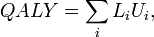
where i is an index of all different time periods, L is the duration of a time period, and U is the utility of health during that time perios (1 = perfect health, 0 = death). QALYs can be calculated for a single person or a population.

Rationale

The QALY is often used in cost-utility analysis in order to estimate the cost-per-QALY associated with a health care intervention. This incremental cost-effectiveness ratio (ICER) can then be used to allocate healthcare resources, often using a threshold approach.

In the United Kingdom, the National Institute for Health and Care Excellence, which advises on the use of health technologies within the National Health Service, has since at least 2013 used "£ per QALY" to evaluate their utility.

The QALY is a measure of the value of health outcomes. Since health is a function of length of life and quality of life, the QALY was developed as an attempt to combine the value of these attributes into a single index number. The basic idea underlying the QALY is simple: it assumes that a year of life lived in perfect health is worth 1 QALY (1 Year of Life × 1 Utility value = 1 QALY) and that a year of life lived in a state of less than this perfect health is worth less than 1. In order to determine the exact QALY value, it is sufficient to multiply the utility value associated with a given state of health by the years lived in that state. QALYs are therefore expressed in terms of "years lived in perfect health": half a year lived in perfect health is equivalent to 0.5 QALYs (0.5 years × 1 Utility), the same as 1 year of life lived in a situation with utility 0.5 (e.g. bedridden) (1 year × 0.5 Utility). QALYs can then be incorporated with medical costs to arrive at a final common denominator of cost/QALY. This parameter can be used to develop a cost-effectiveness analysis of any treatment. Therefore,

QALY is similar to disability-adjusted life year, but the methods of calculation differ.

References

http://heande.opasnet.org/wiki/Talk:Population_attributable_fraction#E-mail_correspondence_between_Jos_Lelieveld.2C_John_Evans.2C_and_Peter_Morfeld

[1] Reference to the Lim Lancet article

[rockhill-2] 1.0 ^1.1 ^1.2 ^1.3 ^1.4 Rockhill B, Newman B, Weinberg C. use and misuse of population attributable fractions. American Journal of Public Health 1998: 88 (1) 15-19.[1]

[3] Kenneth J. Rothman, Sander Greenland, Timothy L. Lash: Modern Epidemiology. Lippincott Williams & Wilkins, 2008. 758 pages.

[darrow-4] 3.0 ^3.1 ^3.2 Darrow LA, Steenland NK. Confounding and bias in the attributable fraction. Epidemiology 2011: 22 (1): 53-58. [2] doi:10.1097/EDE.0b013e3181fce49b

[walter-5] Walter SD. The estimation and interpretation of attributable fraction in health research. Biometrics. 1976;32:829-849.

[kleinbaum-6] 5.0 ^5.1 ^5.2 Kleinbaum DG, Kupper LL, Morgenstem H. Epidemiologic Research. Belmont, Calif: Lifetime Learning Publications; 1982:163.

[miettinen-7] 6.0 ^6.1 Miettinen 0. Proportion of disease caused or prevented by a given exposure, trait, or intervention. Am JEpidemiol. 1974;99:325-332.

[schlesselman-8] 7.0 ^7.1 Schlesselman JJ. Case-Control Studies: Design, Conduct, Analysis. New York, NY: Oxford University Press Inc; 1982.

[bruzzi-9] Bruzzi P, Green SB, Byar DP, Brinton LA, Schairer C. Estimating the population attributable risk for multiple risk factors using case-control data. Am J Epidemiol. 1985; 122: 904-914.

[10] WHO: Health statistics and health information systems. [3]. Accessed 16 Nov 2013.

[robins-11] 10.0 ^10.1 ^10.2 ^10.3 Robins JM, Greenland S. Estimability and estimation of excess and etiologic fractions. Statistics in Medicine 1989 (8) 845-859.

[lelieveld-12] 1.0 ^1.1 Lelieveld J, Evans JS, Fnais M, Giannadaki D, Pozzer A. The contribution of outdoor air pollution sources to premature mortality on a global scale. Nature. 2015 Sep 17;525(7569):367-71. doi:10.1038/nature15371 [4].

[gbd2010-13] 2.0 ^2.1 Lim et al. A comparative risk assessment of burden of disease and injury attributable to 67 risk factors and risk factor clusters in 21 regions, 1990–2010: a systematic analysis for the Global Burden of Disease Study 2010. The Lancet Volume 380, No. 9859, p2224–2260, 15 December 2012. doi:10.1016/S0140-6736(12)61766-8 [5]

[darrow-14] 1.0 ^1.1 ^1.2 Darrow LA, Steenland NK. Confounding and bias in the attributable fraction. Epidemiology 2011: 22 (1): 53-58. [6] doi:10.1097/EDE.0b013e3181fce49b

[burnett-15] Burnett, R. T. et al. An integrated risk function for estimating the Global Burden of Disease attributable to ambient fine particulate matter exposure. Environ. Health Perspect. 122, 397–403 (2014).

[16] Tuomisto, Jouni T.; Pohjola, Mikko; Pohjola, Pasi. Avoin päätöksentekokäytäntö voisi parantaa tiedon hyödyntämistä. [Open policy practice could improve knowledge use.] Yhteiskuntapolitiikka 1/2014, 66-75. http://urn.fi/URN:NBN:fi-fe2014031821621

[17] Pohjola MV, Leino O, Kollanus V, Tuomisto JT, Gunnlaugsdóttir H, Holm F, Kalogeras N, Luteijn JM, Magnússon SH, Odekerken G, Tijhuis MJ, Ueland O, White BC, Verhagen H. State of the art in benefit-risk analysis: Environmental health. Food Chem Toxicol. (2012) 50: 1: 40-55. [7]

[18] Tuomisto JT. Massadata kansanterveyden edistämisessä. [Big data in promotion of public health.] Duodecim 2015;131:2179–87. URN:NBN:fi-fe201601071478

[19] Havelaar A., De Hollander A.E.M., Teunis P.F.M., Evers E.G., Van Kranen H.J., Versteegh J.F.M., Van Koten J.E.M., Slob W. Balancing the Risks and Benefits of Drinking Water Disinfection : Disabiliity Adjusted Life-Years on the Scale. Environ Health Perspect 108:315-321 (2000)

[20] Knol, A.B. en Staatsen, B.A.M. (2005). Trends in the environmental burden of disease in the Netherlands, 1980-2020. Rapport 500029001, RIVM, Bilthoven. Downloadable at http://www.rivm.nl/bibliotheek/rapporten/500029001.html

[1]

[1]

[2]

[3]

[4]

[5]

[6]

[7]

[8]

[9]

[10]

[1]

[2]

[1]

[2]

[1]

[2]

[3]

[1]

[2]

Binding scientific information production, critique, and use

Contents

Disease burden method

Question

Answer

Rationale

Global Burden of Disease Study 2010

Calculations

See also

Keywords

References

Health indicator method

Question

Answer

Rationale

DALY

QALY

Number of cases

Life expectancy

Welfare indicators

See also

References

Attributable risk method

Question

Answer

Rationale

Excess fraction

Impact of confounders

Population attributable fraction

Etiologic fraction

Calculations

See also

References

Discussion about attributable risk method

Scientific disputes possibly related to attributable risk

Response to Morfeld and Erren Int J Public Health

References

Greenland 1999

Choosing the right fraction

Meaning of premature

Abstract to ISEE, Rome 2016

Travel report

Study on disease burden of air pollution

Question

Answer

Rationale

Interpretation

Data

Lelieveld2015 disease burden methods

See also

Keywords

References

Related files

Discussion on the study

Value judgements by Lelieveld2015

Case-specific values

Generic health indiator advice

Case-specific advice

Bias in attributable fraction

Exposed population

Confounding in RR

Overall bias

References

Knowledge crystal method

Question

Answer

Rationale

Different information objects and their usage

Producing shared understanding by utilising knowledge crystals

Additional methods: DALY

Question

Answer

Rationale

Integrated health measures

Parameters

Uncertainty

Appendix: common integrated health measures

Mortality figures

Morbidity figures

Healthy life expectancy